Perturbation Theory – Case Study 1

Since then, we have presented some methods to sum series (Padé approximants, Euler summation, Borel summation, Borel-Écalle summation, generic summation and Zeta summation). We have also seen techniques to accelerate convergence (Shanks transformation and Richardson transformation).

When a problem is not solvable exactly (extracting the roots of a polynomial, solving a specific differential equation, …) the idea of perturbation theory is to obtain an approximate solution (analytically) by inserting a small parameter \epsilon and assuming the answer has the form a_0 + a_1 \epsilon + a_2 \epsilon^2 + a_3 \epsilon^3 + \dots.

Procedure:

  • Insert \displaystyle \epsilon
  • Set \displaystyle \epsilon = 0 (the problem must be exactly solvable for \displaystyle \epsilon = 0)
  • The solution has the form \displaystyle x_{\epsilon} = a_0 + a_1 \epsilon + a_2 \epsilon^2 + a_3 \epsilon^3 + \dots
  • Set \displaystyle \epsilon = 1 (the solution of the initial problem is now \displaystyle a_0 + a_1 + a_2 + a_3 + \dots)
  • Study the convergence of \displaystyle a_0 + a_1 + a_2 + a_3 + \dots
  • If necessary use a summation method

Solve a very simple ‘problem’ using perturbation theory:

\displaystyle x - 2 = 0 \quad \text{Problem}
\displaystyle x - 2\epsilon = 0 \quad \text{Insert } \epsilon
\displaystyle (a_0 + a_1 \epsilon + a_2 \epsilon^2 + \dots) - 2\epsilon = 0 \quad \text{Insert } x_{\epsilon}
\displaystyle a_0 + (a_1 - 2)\epsilon + a_2 \epsilon^2 + \dots = 0 + 0 + 0 + \dots

Because coefficients of Taylor series are unique (see proof) we are allowed to compare powers of \epsilon.

\displaystyle \implies a_0 = 0,\ a_1 = 2,\ a_2 = 0,\ \dots
\displaystyle x_{\epsilon} = 0 + 2\epsilon + 0 + \dots
\displaystyle x_{\epsilon} = 2\epsilon

This implies that x = 2 (setting \epsilon = 1).

In the figure below, we visualize the solution of x - 2\epsilon = 0 as a function of \epsilon.


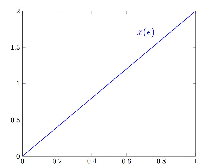
Solution of the problem x - 2 = 0 using perturbation theory. For \epsilon = 0 the solution is zero and for \epsilon = 1 the solution is 2. By making \epsilon approach 1 we obtain an increasingly precise answer to the initial problem.

Comments

Leave a comment