Let’s imagine we don’t have a calculating machine or computer and we want to calculate the value of the root of 2 using perturbation theory. Remember that we always insert epsilon so that the problem is exactly solvable for epsilon equals zero. Here’s how we might proceed:
In this case, we keep only the powers of epsilon up to order two. We want to perform a perturbative calculation of order two.
Let us solve the same problem but this time we keep the powers of epsilon up to order three.
This suggests the following (using the double factorial notation):
We could use Euler’s summation to speed up the convergence of this series. We observe that perturbing the initial problem in this form:
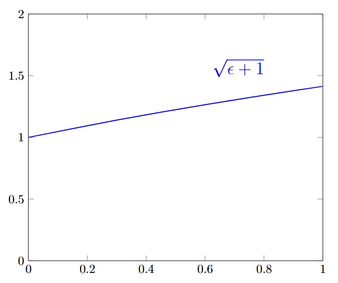
Evaluating the solution at recovers the original problem and gives . In the figure below we visualize the solution of as a function of .
For this very simple example, we essentially chose a placement of such that the unperturbed problem (for ) becomes trivial. We also have many choices for the power of . In this example, the perturbation series terminates and yields the exact solution.
Since then, we have presented some methods to sum series (Padé approximants, Euler summation, Borel summation, Borel-Écalle summation, generic summation and Zeta summation). We have also seen techniques to accelerate convergence (Shanks transformation and Richardson transformation).
When a problem is not solvable exactly (extracting the roots of a polynomial, solving a specific differential equation, …) the idea of perturbation theory is to obtain an approximate solution (analytically) by inserting a small parameter and assuming the answer has the form .
Procedure:
Insert
Set (the problem must be exactly solvable for )
The solution has the form
Set (the solution of the initial problem is now )
Study the convergence of
If necessary use a summation method
Solve a very simple ‘problem’ using perturbation theory:
Because coefficients of Taylor series are unique (see proof) we are allowed to compare powers of .
This implies that (setting ).
In the figure below, we visualize the solution of as a function of .
Solution of the problem using perturbation theory. For the solution is zero and for the solution is 2. By making approach 1 we obtain an increasingly precise answer to the initial problem.
In physics, most problems—from the anharmonic oscillator to Quantum Electrodynamics (QED)— cannot be solved exactly. We rely on Perturbation Theory, expanding the solution in powers of a small coupling constant (often denoted λ or α).
A classic example is the quantum anharmonic oscillator, where the Hamiltonian is
(with the quartic term treated as a small perturbation λ ≪ 1). Another famous case is QED, where the fine-structure constant α ≈ 1/137 serves as the small parameter for expanding processes involving electrons and photons.
The challenge? These perturbative expansions are almost always asymptotic series with a null radius of convergence. The coefficients typically grow factorially as (or even faster), making the series eventually diverge regardless of how small the coupling constant is.
For instance, in the anharmonic oscillator, the perturbative corrections to the energy levels involve terms whose coefficients grow like , leading to a divergent series for any nonzero λ. Similarly, in QED, the perturbative series for quantities like the electron’s anomalous magnetic moment (g−2) is asymptotic: it gives spectacular agreement with experiment up to high orders, but diverges if pushed too far.
This is where our journey pays off. By applying Borel resummation and Padé approximants to these divergent series, we can extract non-perturbative information and obtain remarkably accurate physical predictions. In quantum field theory, Borel summation helps recover meaningful results from perturbative expansions (for example, in certain Euclidean field theories or by handling contributions from instantons and renormalons). Padé approximants are routinely used to accelerate convergence and estimate the behavior of series in QCD and other models.
In our upcoming posts, we will see how this mathematical framework becomes the essential language of modern theoretical physics.
After several months of exploring various summation and acceleration methods, it is time to synthesize these tools before we apply them to one of their most important domains: Perturbation Theory.
When a power series has a small or even zero radius of convergence, or converges too slowly to be numerically useful, we require more than standard arithmetic. Here is a recap of the methods we have covered and how they bridge the gap between formal series and numerical values.
Summation Methods: Taming Divergence
Borel and Borel–Écalle: By using the Borel transform, we transform factorially growing coefficients into a convergent series in the Borel plane. The Borel–Écalle framework further allows us to handle singularities via resurgence theory, providing a unique “resummed” value even for non-Borel-summable series.
Euler and Zeta summation: These methods assign finite values to divergent sums by analytic continuation. While Euler summation is ideal for alternating series, Zeta summation provides a powerful way to handle the infinite sums that frequently appear in quantum vacuum energy calculations.
Generic summation: Beyond these classical approaches, we have also explored the idea of generic summation, which provides a unifying framework for assigning values to divergent or slowly convergent series.
Acceleration Techniques: Enhancing Convergence
Shanks Transformation and Padé Approximants: These nonlinear transformations (often related to continued fractions) excel at capturing the behavior of functions beyond their radius of convergence, particularly when poles are present.
Richardson Extrapolation: A fundamental tool for numerical analysis that cancels out the leading error terms, allowing us to estimate the limit of a sequence Sn with much higher precision from only a few terms.
An important consistency check underlies all these techniques: whenever different summation or acceleration methods apply to the same series, they agree on a common value. This convergence of independent approaches is not accidental, it reflects the fact that these methods capture an underlying analytic object beyond the formal series itself. When they work, they do not merely assign a value: they reveal a coherent extension of the function that the original divergent expansion was hinting at.


 :
:


 recovers the original problem and gives
  . In the figure below we visualize the solution of
  as a function of
  ) becomes trivial. We also have many choices for the power of
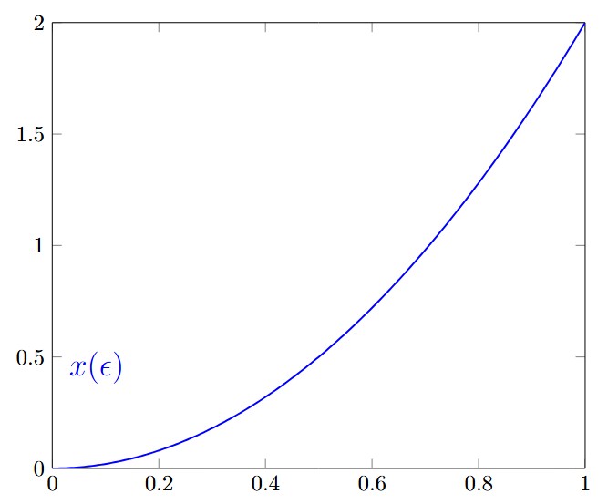
 .
.
 (the problem must be exactly solvable for
 (the solution of the initial problem is now
  )
)


 as a function of
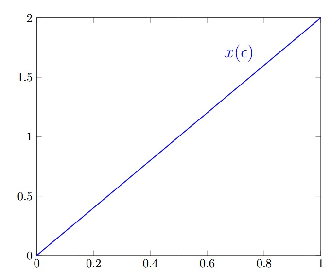
 using perturbation theory. For
 typically grow factorially as
  (or even faster), making the series eventually diverge regardless of how small the coupling constant is.
 has a small or even zero radius of convergence, or converges too slowly to be numerically useful, we require more than standard arithmetic. Here is a recap of the methods we have covered and how they bridge the gap between formal series and numerical values.