Regular Problem I

Written by

In perturbation theory we distinguish regular and singular problems. In this section we aim to solve the original regular problem:

$\displaystyle x^2 - 2 = 0 \quad \text{Original problem}$

$\displaystyle x^2 - (1 + \epsilon) = 0 \quad \text{Insert epsilon}$

The solutions are:

$\displaystyle x_1(\epsilon) = -\sqrt{1+\epsilon}$

$\displaystyle x_2(\epsilon) = \sqrt{1+\epsilon}$

At $\epsilon=0$ the problem is solvable analytically:

$\displaystyle x_1 = -1, \quad x_2 = 1$

At $\epsilon=1$ we recover the solution of the original problem:

$\displaystyle x_1 = -\sqrt{2}, \quad x_2 = \sqrt{2}$

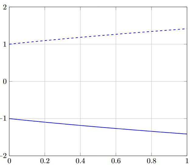
Figure. Regular problem: $x^2-(1+\epsilon)=0$ connecting $x^2-1=0$ to $x^2-2=0$ .

Characteristics of a regular perturbation problem:

The solution depends smoothly on ε.
The deformation from ε=0 to ε=1 is continuous.
The problem at ε=0 is simple and solvable analytically.
The original problem is recovered exactly at ε=1.
No singularities or discontinuities appear.
The solution admits a regular power-series expansion in ε.

We treat $\epsilon$ as a parameter to track the perturbation. The solution $x_2(\epsilon) = \sqrt{1+\epsilon}$ can be expressed as a Taylor series around the simple problem ( $\epsilon = 0$ ):

$\displaystyle x_2(\epsilon) = 1 + \frac{1}{2}\epsilon - \frac{1}{8}\epsilon^2 + \frac{1}{16}\epsilon^3 - \frac{5}{128}\epsilon^4 + \dots$

The original problem $x^2 - 2 = 0$ is recovered by evaluating this series at $\epsilon = 1$ . The smooth dependence on the parameter allows us to reach the target solution. For $\epsilon=1$ , the first few terms give: