Month: May 2026

Regular Problem II

Illustration of another regular problem:

$\displaystyle x^2-2x -1 = 0 \quad \text{Problem}$

$\displaystyle x^2-2\epsilon x-1=0 \quad \text{Insert }\epsilon$

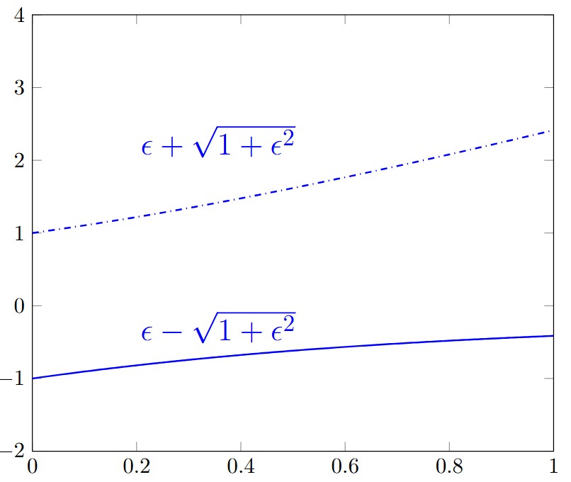
The solutions to the perturbed problem are (see figure below):

$\displaystyle x_1(\epsilon) = \frac{2\epsilon + \sqrt{4 \epsilon^2 + 4}}{2} = \epsilon + \sqrt{1 + \epsilon^2}$

$\displaystyle x_2(\epsilon) = \frac{2\epsilon - \sqrt{4 \epsilon^2 + 4}}{2} = \epsilon - \sqrt{1 + \epsilon^2}$

The figure above shows solutions of the problem $x^2-2\epsilon x-1 = 0$ using perturbation theory. For $\epsilon =0$ the solutions are -1 and 1 and for $\epsilon =1$ the solutions are exactly $1+\sqrt{2}$ and $1-\sqrt{2}$ .

$\displaystyle x_1(\epsilon) = 1 + \epsilon + \frac{1}{2}\epsilon^2 - \frac{1}{8}\epsilon^4 + \frac{1}{16}\epsilon^6 - \frac{5}{128}\epsilon^8 + O(\epsilon^{10})$

$\displaystyle x_2(\epsilon) = -1 + \epsilon - \frac{1}{2}\epsilon^2 + \frac{1}{8}\epsilon^4 - \frac{1}{16}\epsilon^6 + \frac{5}{128}\epsilon^8 + O(\epsilon^{10})$

Setting $\epsilon = 1$ :

$\displaystyle x_1(1) \approx 2 + \frac{1}{2} - \frac{1}{8} + \frac{1}{16} - \frac{5}{128} = 2.3984375$

$\displaystyle x_2(1) \approx 0 - \frac{1}{2} + \frac{1}{8} - \frac{1}{16} + \frac{5}{128} = -0.3984375$

This simple example clearly illustrates the application of regular perturbation theory to a quadratic equation, showing how the solutions vary continuously with the perturbation parameter $\epsilon$ .

May 28, 2026
Regular Problem I
In perturbation theory we distinguish regular and singular problems. In this section we aim to solve the original regular problem:

$\displaystyle x^2 - 2 = 0 \quad \text{Original problem}$

$\displaystyle x^2 - (1 + \epsilon) = 0 \quad \text{Insert epsilon}$

The solutions are:

$\displaystyle x_1(\epsilon) = -\sqrt{1+\epsilon}$

$\displaystyle x_2(\epsilon) = \sqrt{1+\epsilon}$

At $\epsilon=0$ the problem is solvable analytically:

$\displaystyle x_1 = -1, \quad x_2 = 1$

At $\epsilon=1$ we recover the solution of the original problem:

$\displaystyle x_1 = -\sqrt{2}, \quad x_2 = \sqrt{2}$

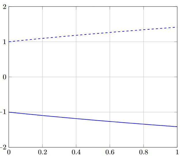
Figure. Regular problem: $x^2-(1+\epsilon)=0$ connecting $x^2-1=0$ to $x^2-2=0$ .

Characteristics of a regular perturbation problem:
- The solution depends smoothly on ε.
- The deformation from ε=0 to ε=1 is continuous.
- The problem at ε=0 is simple and solvable analytically.
- The original problem is recovered exactly at ε=1.
- No singularities or discontinuities appear.
- The solution admits a regular power-series expansion in ε.
We treat $\epsilon$ as a parameter to track the perturbation. The solution $x_2(\epsilon) = \sqrt{1+\epsilon}$ can be expressed as a Taylor series around the simple problem ( $\epsilon = 0$ ):

$\displaystyle x_2(\epsilon) = 1 + \frac{1}{2}\epsilon - \frac{1}{8}\epsilon^2 + \frac{1}{16}\epsilon^3 - \frac{5}{128}\epsilon^4 + \dots$

The original problem $x^2 - 2 = 0$ is recovered by evaluating this series at $\epsilon = 1$ . The smooth dependence on the parameter allows us to reach the target solution. For $\epsilon=1$ , the first few terms give:

$\displaystyle x_2(1) \approx 1 + 0.5 - 0.125 + 0.0625 - 0.039 = 1.3985$

which is already a good approximation $\sqrt{2} \approx 1.4142$ .

This example illustrates a regular homotopy connecting the simple problem $x^2 - 1 = 0$ to the target problem $x^2 - 2 = 0$ .
May 21, 2026

Polynomial expansion

Expanding series and sorting coefficients by hand can be tedious. The Python library sympy allows us to automate this process efficiently.

Polynomial expansion and coefficient extraction

from sympy import symbols, expand, collect

# define variables
a0, a1, a2, a3, x = symbols('a0 a1 a2 a3 x')

# expand the expression
expr = expand((a0 + a1*x + a2*x**2 + a3*x**3)**2)

print("Expanded expression:")
print(expr)

print("\nCollected by powers of x:")
print(collect(expr, x))

Output:

Expanded expression:
a0**2 + 2*a0*a1*x + 2*a0*a2*x**2 + 2*a0*a3*x**3
+ a1**2*x**2 + 2*a1*a2*x**3 + 2*a1*a3*x**4
+ a2**2*x**4 + 2*a2*a3*x**5 + a3**2*x**6

Collected by powers of x:
a0**2 + 2*a0*a1*x
+ (2*a0*a2 + a1**2)*x**2
+ (2*a0*a3 + 2*a1*a2)*x**3
+ (2*a1*a3 + a2**2)*x**4
+ 2*a2*a3*x**5
+ a3**2*x**6

We can also extract coefficients order by order:

coeffs = [expr.coeff(x, i) for i in range(7)]

for i, c in enumerate(coeffs):
    print(f"Coefficient of x^{i}:", c)

Output:

Coefficient of x^0: a0**2
Coefficient of x^1: 2*a0*a1
Coefficient of x^2: 2*a0*a2 + a1**2
Coefficient of x^3: 2*a0*a3 + 2*a1*a2
Coefficient of x^4: 2*a1*a3 + a2**2
Coefficient of x^5: 2*a2*a3
Coefficient of x^6: a3**2

This approach allows us to systematically extract and match coefficients order by order, which is particularly useful in perturbation theory.

May 14, 2026

sqrt(2) bis

Let us revisit the problem of computing the value of $\sqrt{2}$ , but this time we slightly modify our perturbative approach to improve convergence.

Previously, we expanded around $x=1$ , which is relatively far from the true value. Instead, we now choose a better starting point.

$\displaystyle x = \sqrt{2} \quad \text{Problem}$

We observe that:

$\displaystyle \left(\frac{3}{2}\right)^2 = \frac{9}{4} = 2.25 \quad \text{so it is close to } 2$

This suggests writing:

$\displaystyle x = \frac{3}{2} + \delta$

The correction $\delta$ is expected to be small, which improves the convergence of the perturbative expansion.

We now insert this into the equation:

$\displaystyle x^2 = 2$

$\displaystyle \left(\frac{3}{2} + \delta \right)^2 = 2$

$\displaystyle \frac{9}{4} + 3\delta + \delta^2 = 2$

Rearranging, we obtain:

$\displaystyle 3\delta + \delta^2 = -\frac{1}{4}$

We now introduce a perturbation parameter $\epsilon$ :

$\displaystyle 3\delta + \delta^2 = -\frac{1}{4}\varepsilon$

We seek a solution of the form:

$\displaystyle \delta = b_1 \varepsilon + b_2 \varepsilon^2 + b_3 \varepsilon^3 + \cdots$

Substituting into the equation and expanding:

$\displaystyle 3b_1\varepsilon + 3b_2\varepsilon^2 + b_1^2\varepsilon^2 + \cdots = -\frac{1}{4}\varepsilon$

Matching powers of $\varepsilon$ :

$\displaystyle \varepsilon^1: \quad 3b_1 = -\frac{1}{4} \Rightarrow b_1 = -\frac{1}{12}$

$\displaystyle \varepsilon^2: \quad 3b_2 + b_1^2 = 0 \Rightarrow b_2 = -\frac{1}{432}$

Thus:

$\displaystyle \delta = -\frac{1}{12}\varepsilon - \frac{1}{432}\varepsilon^2 + \cdots$

We finally obtain:

$\displaystyle x = \frac{3}{2} - \frac{1}{12}\varepsilon - \frac{1}{432}\varepsilon^2 + \cdots$

Setting $\varepsilon = 1$ :

$\displaystyle x \approx \frac{3}{2} - \frac{1}{12} - \frac{1}{432} = 1.41435$

which is already a very good approximation of $\sqrt{2} \approx 1.41421$ .

This example illustrates a key idea in perturbation theory:

The choice of the unperturbed problem strongly affects the convergence of the series.

By expanding around a value closer to the true solution, we obtain a much more efficient approximation with fewer terms.

May 7, 2026