Category: Uncategorized

  • Asymptotics: Motivation

    To make progress in perturbation theory, we need to introduce the notion of ‘asymptotic series’. To introduce this concept, we’ll consider the following integral:

    \displaystyle I(x) = \int_{0}^{\infty} \frac{e^{-xt}}{1+t}\, dt \quad (\mathrm{Re}(x) > 0)

    Using

    \displaystyle \frac{1}{1+t} = 1-t+t^2-t^3+\cdots, \qquad |t|<1

    we obtain the asymptotic expansion

    \displaystyle I(x) \sim \frac{0!}{x}-\frac{1!}{x^2}+\frac{2!}{x^3}-\cdots
    \displaystyle I(x) \sim \sum_{n=0}^{\infty}(-1)^n\frac{n!}{x^{n+1}}, \qquad x\to+\infty

    This series is divergent for all x\neq 0, since its terms do not tend to zero. Let us evaluate the first 5 terms of the series for x=10 and compare the result to a numerical solution I(10)\approx 0.09156:

    \displaystyle 0.1-0.01+0.002-0.0006+0.00024=0.09164

    We observe that the first 5 terms of the divergent series give a good approximation of the value obtained using numerical methods. We find ourselves in the case of astronomers’ series as presented by H. Poincaré.

    We can ask ourselves how many terms we need to use to achieve a certain level of accuracy in our calculations. To do this, we reformulate the integral above using a partial sum and a remainder R_n(x):

    \displaystyle I(x)=\sum_{k=0}^{n-1}(-1)^k\frac{k!}{x^{k+1}}+R_n(x)

    where

    \displaystyle R_n(x)=I(x)-\sum_{k=0}^{n-1}(-1)^k\frac{k!}{x^{k+1}}

    The remainder term can be seen as the error made by stopping after n terms. We would like to estimate the remainder:

    \displaystyle \frac{1}{1+t}=\sum_{k=0}^{n-1}(-1)^k t^k+\frac{(-1)^n t^n}{1+t}

    Therefore,

    \displaystyle I(x)=\int_0^\infty e^{-xt}\left(\sum_{k=0}^{n-1}(-1)^k t^k\right)\,dt+\int_0^\infty\frac{(-1)^n t^n e^{-xt}}{1+t}\,dt

    The remainder is

    \displaystyle R_n(x) = \int_{0}^{\infty} \frac{(-1)^n t^n e^{-xt}}{1+t}\, dt
    \displaystyle |R_n(x)| = \int_{0}^{\infty} \frac{t^n e^{-xt}}{1+t}\, dt
    \displaystyle |R_n(x)| < \int_{0}^{\infty} t^n e^{-xt}\, dt
    \displaystyle \int_{0}^{\infty} t^n e^{-xt}\, dt = \frac{n!}{x^{n+1}}, \quad x > 0

    We observe that \frac{n!}{x^{n+1}} is the first omitted term in the series, so that the remainder is smaller than the first omitted term. The term \frac{n!}{x^{n+1}} decreases but then eventually gets bigger. We have to stop after some terms. For example, for x=10, the terms of minimum magnitude occur at indices n=9 and n=10, so we can truncate after either 10 or 11 terms.

    The series

    \displaystyle \frac{0!}{x}-\frac{1!}{x^2}+\frac{2!}{x^3}-\cdots

    provides a useful approximation for I(x) for large x. This series is called an asymptotic series.

  • Stieltjes functions in physics

    Stieltjes functions arise naturally in physics when linear differential operators with positive spectra lead to observable quantities that admit positive spectral representations.

    This structure makes Padé approximants particularly powerful, enabling accurate physical predictions from perturbation series or spectral data, even when conventional methods fail.

    Here are three examples of fields in physics where Stieltjes functions play an important role and Padé approximants provide powerful approximation techniques:

    1. Quantum anharmonic oscillator: The perturbation series for the ground-state energy of the quartic anharmonic oscillator diverges factorially at large order. Nevertheless, its Stieltjes structure provides a rigorous foundation for Padé approximation, allowing highly accurate energy estimates to be obtained from perturbative coefficients, even at strong coupling. This is an example of how a divergent series can encode remarkably precise physical information.
    2. Composite materials:
      Predicting the effective dielectric constant or electrical conductivity of heterogeneous materials is a challenging problem, since the macroscopic response depends on the microscopic structure of the constituents. Through the spectral representations developed in Bergman–Milton theory, these effective properties can, under appropriate assumptions, be expressed as Stieltjes functions of the contrast between the constituent materials. Padé approximants and related methods can then provide accurate estimates and rigorous bounds on the effective properties.
    3. Atomic and molecular polarizabilities:
      The frequency-dependent dipole polarizability of atoms and molecules admits a spectral representation in terms of excitation energies and oscillator strengths. Under the usual assumptions, this gives rise to a Stieltjes structure in the squared frequency. The associated moment problem is the foundation of the Stieltjes imaging technique, which uses Padé-related approximations to reconstruct photoabsorption spectra and photoionization cross sections from discrete variational calculations.

    Despite their different physical origins, these examples share a common mathematical structure: positive spectral representations make it possible to exploit the special properties of Stieltjes functions and the convergence behavior of Padé approximants.

  • Stieltjes functions II

    In the previous post, we studied the direct problem of constructing a Stieltjes function from a given weight function and explored the associated Stieltjes series and Padé approximants. Now, let’s consider the opposite problem and first define the weight function. In this case, we choose:

    \displaystyle \rho(t)=\begin{cases}1 & \text{if } 0 < t < 1 \\ 0 & \text{otherwise}\end{cases}

    this implies that

    \displaystyle a_n = \int_{0}^{\infty} \rho(t) t^n \, dt
    \displaystyle = \int_{0}^{1} t^n \, dt = \frac{1}{n+1}

    This implies that the corresponding Stieltjes series is (see previous post):

    \displaystyle \sum_{n=0}^{\infty} \frac{(-1)^n x^n}{n+1}

    (which has radius of convergence 1 and coincides with f(x) for |x|<1) and the Stieltjes function is:

    \displaystyle f(x) = \frac{\log(1+x)}{x}

    (where \log denotes the principal branch, with cut along (-\infty,-1]). Thus f is analytic in \mathbb{C}\setminus(-\infty,-1].

    Properties of Stieltjes functions:

    • f(x) is analytic in the cut complex plane \mathbb{C}\setminus(-\infty,0] (in the present example the natural cut is actually shorter: \mathbb{C}\setminus(-\infty,-1]).

    • f(x)\ge 0 for all x>0.

    • f(x) \to 0 as |x| \to \infty in the cut complex plane, under appropriate assumptions on \rho(t).

    • f(x) \sim \sum_{n=0}^{\infty} (-1)^n a_n x^n as |x| \to 0 in the cut complex plane.

    • -f(x) is Herglotz (i.e., \mathrm{Im}(-f(x)) has the same sign as \mathrm{Im}(x)).

    Under appropriate additional hypotheses, a converse characterization also holds: a function satisfying the corresponding analyticity, asymptotic, positivity, and Herglotz properties is a Stieltjes function. It can be proved rigorously that appropriate Padé approximants of a Stieltjes series converge. This is a particularly useful result (which we have already illustrated with examples), as it implies that the Padé approximants constructed from the Stieltjes series converge to the Stieltjes function for x in the cut complex plane, under appropriate hypotheses.

  • Stieltjes function I

    The function f(x) is a Stieltjes function if it has the following form:

    \displaystyle f(x) = \int_{0}^{\infty} \frac{\rho(t)}{1+xt} \, dt

    where \rho(t) is a ‘weight function’ with \rho(t) \geq 0 for all 0 \leq t < \infty and the moments of \rho(t) exist. The moments are defined as:

    \displaystyle a_n = \int_{0}^{\infty} \rho(t) t^n \, dt

    Using the geometric series expansion of \frac{1}{1 + xt}, the Stieltjes function has the following asymptotic expansion:

    \displaystyle f(x) = \int_{0}^{\infty} \frac{\rho(t)}{1+xt} \, dt \sim \int_{0}^{\infty} \sum_{n=0}^{\infty} (-1)^n x^n t^n \rho(t) \, dt
    \displaystyle = \sum_{n=0}^{\infty} (-1)^n \left( \int_{0}^{\infty} \rho(t) t^n \, dt \right) x^n
    \displaystyle = \sum_{n=0}^{\infty} (-1)^n a_n x^n

    This series is called a ‘Stieltjes series’ and is often divergent since the moments a_n can grow sufficiently rapidly for the series to have zero radius of convergence. Let begin the exploration of Stieltjes functions with an example. Let set \rho(t) = e^{-t}. We have:

    \displaystyle f(x) = \int_{0}^{\infty} \frac{e^{-t}}{1+xt} \, dt
    \displaystyle \sim \sum_{n=0}^{\infty} (-1)^n \left( \int_{0}^{\infty} e^{-t} t^n \, dt \right) x^n
    \displaystyle = \sum_{n=0}^{\infty} (-1)^n n! x^n

    So \rho(t) = e^{-t} \implies a_n = n!.

    Stieltjes functions and their associated series offer a classic illustration of how divergent asymptotic expansions can still encode precise analytic information, a theme that continues to play a central role in asymptotic analysis and resurgence theory.

  • Padé to the Rescue

    Recall that in the previous posts we attempted to calculate the following Stieltjes integral using perturbation techniques:

    \displaystyle I(\epsilon) = \int_{0}^{\infty} \frac{e^{-t}}{1 + \epsilon^2 t}\,dt

    For \epsilon = 1, we obtain the target integral I(1) = \int_{0}^{\infty} \frac{e^{-t}}{1+t}\,dt. Expanding (1 + \epsilon^2 t)^{-1} as a formal power series and integrating term by term leads to the series:

    \displaystyle \sum_{k=0}^{\infty} (-1)^{k} k! \, \epsilon^{2k}

    This series is divergent for \epsilon = 1 and does not allow us to directly approximate the exact value of the integral. We can, however, approximate the exact value using Padé approximants. By making the change of variable x = \epsilon^2, the series transforms into a dense power series in x, \sum_{k=0}^{\infty} (-1)^{k} k! \, x^k. We then construct its diagonal Padé approximants [N/N](x) evaluated at x = 1.

    The following R code calculates and evaluates the [5/5] Padé approximant using the pracma package (note: coefficients must be supplied in decreasing order of powers for pracma::pade):

    library(pracma)
    
    # Series coefficients a_k = (-1)^k * k! in DECREASING order of powers
    k <- 10:0
    p1 <- (-1)^k * factorial(k)
    
    # Compute [5/5] Pade approximant with respect to x = epsilon^2
    Q  <- pade(p1, d1 = 5, d2 = 5)
    r1 <- Q$r1
    r2 <- Q$r2
    
    # Rational function evaluation
    f1 <- function(x) polyval(r1, x) / polyval(r2, x)
    
    # Evaluate at epsilon = 1 (x = 1^2 = 1)
    f1(1)
    
    # Plot graph
    xs <- seq(-1, 1, length.out=100)
    ys1 <- f1(xs)
    plot(xs, ys1, type = "l", col="blue", xlab="x", ylab="P[5,5](x)")
    grid()

    In the table below, the values of successive diagonal Padé approximants [N/N](x) evaluated at x = 1 are displayed. We can observe that these values converge rapidly towards the exact value of the integral (I \approx 0.596347).

    Padé approximants have therefore made it possible to evaluate a Stieltjes integral represented by a divergent series. This result can be extended to the class of all Stieltjes functions, which will be the subject of the next posts

    Padé [N/N] Padé approximant Approximation at x = 1 Error
    [1/1] (1 + x)/(1 + 2x) 0.666667 7.03 × 10⁻²
    [2/2] (1 + 5x + 2x2)/(1 + 6x + 6x2) 0.615385 1.90 × 10⁻²
    [3/3] (1 + 11x + 26x2 + 6x3)/(1 + 12x + 36x2 + 24x3) 0.602740 6.39 × 10⁻³
    [4/4] (1 + 19x + 102x2 + 154x3 + 24x4)/(1 + 20x + 120x2 + 240x3 + 120x4) 0.598802 2.46 × 10⁻³
    [5/5] (1 + 29x + 272x2 + 954x3 + 1044x4 + 120x5)/(1 + 30x + 300x2 + 1200x3 + 1800x4 + 720x5) 0.597383 1.04 × 10⁻³
    [10/10] (exact rational of degree 10) 0.596379 3.15 × 10⁻⁵
  • Stieltjes integral II

    If we give \epsilon the value 1 for the series from the previous post and draw up a table of the values of the integral as a function of n, we can see that the values first converge towards the exact value and then move away from it (see table below). This reminds us of the “astronomers’ series” described by H. Poincaré. We also note that we cannot approach the exact value with arbitrary precision using this method.

    n Approximation Error
    0 1 0.4036
    1 0 -0.5963
    2 2 1.4037
    3 -4 -4.5963
    4 20 19.4037
    5 -100 -100.5963

    Given such a series, a natural question is: Up to what value of n should we sum in order to get as close as possible to the exact value ? In order to determine the ideal value of n, we must first note the following facts concerning the remainder of the series above:

    \displaystyle I_{n+1}(\epsilon) := \int_{0}^{\infty} \frac{e^{-t} t^{n+1}}{1 + \epsilon^2 t} dt
    \displaystyle |I_{n+1}(\epsilon)| > \int_{1}^{\infty} \frac{e^{-t} t^{n+1}}{1 + \epsilon^2 t} dt > \int_{1}^{\infty} \frac{e^{-t} t^{n+1}}{t + \epsilon^2 t} dt

    Defining t := 1+s (\implies dt = ds), we have:

    \displaystyle \int_{1}^{\infty} \frac{e^{-t} t^{n+1}}{t + \epsilon^2 t} dt = \int_{0}^{\infty} \frac{e^{-1-s} (1+s)^{n+1}}{(1+s) + \epsilon^2 (1+s)} ds
    \displaystyle = \frac{e^{-1}}{1 + \epsilon^2} \int_{0}^{\infty} e^{-s} (1+s)^n ds

    We observe that:

    \displaystyle \frac{e^{-1}}{1 + \epsilon^2} \int_{0}^{\infty} e^{-s} (1+s)^n ds > \frac{e^{-1}}{1 + \epsilon^2} \int_{0}^{\infty} e^{-s} s^n ds
    \displaystyle = \frac{e^{-1}}{1 + \epsilon^2}n!

    Therefore:

    \displaystyle |I_{n+1}(\epsilon)| > \frac{e^{-1}}{1 + \epsilon^2}n!
    \displaystyle \epsilon^{2n+2}|I_{n+1}(\epsilon)| > \epsilon^{2n+2}\frac{e^{-1}}{1 + \epsilon^2}n!

    Based on the above calculations, we can now define a lower bound (L_{n+1}(\epsilon)) and an upper bound (U_{n+1}(\epsilon)) for the error made when evaluating the Stieltjes integral using the sum derived above.

    \displaystyle L_{n+1}(\epsilon) := \epsilon^{2n+2}\frac{e^{-1}}{1 + \epsilon^2}n!
    \displaystyle < \left|I_{\epsilon} - \sum_{k=0}^{n} (-1)^k \epsilon^{2k} k!\right|
    \displaystyle < \epsilon^{2n+2} (n+1)! =: U_{n+1}(\epsilon)

    For \epsilon = 1, we have L_{n+1}(\epsilon) = \frac{e^{-1}}{2}n! and U_{n+1}(\epsilon) = (n+1)!. The approximation, error, and corresponding upper and lower bounds for the error are shown for \epsilon = 1 in the table below. In this table, we can clearly see that the approximations are getting worse and worse, while the lower and upper bounds are getting larger and larger. This makes the perturbative method, as implemented in this example, unattractive.

    n Approximation |Error| L_{n+1}(\epsilon) U_{n+1}(\epsilon)
    0 1 0.4036 0.18393 1
    1 0 0.5963 0.18393 2
    2 2 1.4037 0.36788 6
    3 -4 4.5963 1.10364 24
    4 20 19.4037 4.41455 120
    5 -100 100.5963 22.0728 720
  • Stieltjes integral I

    In this post we would like to illustrate the calculation of an integral using perturbation techniques. We would like to calculate the following Stieltjes integral:

    \displaystyle I = \int_{0}^{\infty} \frac{e^{-t}}{1+t}dt

    This integral can be evaluated exactly (I = 0.5963), but we’ll use perturbation techniques to compare the results obtained using these approximation techniques with the exactly calculated value. In order to do so, we will insert the parameter \epsilon as follows:

    \displaystyle I(\epsilon) = \int_{0}^{\infty} \frac{e^{-t}}{1+\epsilon^2t}dt

    For \epsilon = 0 we have I(\epsilon) = 1. This is the solution to the unperturbed problem. We observe that:

    \displaystyle \frac{1}{1-x} = 1 + x + x^2 + ...
    \displaystyle = 1 + x + x^2 + ... + x^n + x^{n+1}(1 + x + x^2 + ...)
    \displaystyle =  1 + x + x^2 + ... + x^n + \frac{x^{n+1}}{1-x}

    Defining x := -\epsilon^2 t and using \int_{0}^{\infty} e^{-t} t^n dt = n! in the formula above we obtain:

    \displaystyle \frac{1}{1 +\epsilon^2t} =  1 -\epsilon^2 t   + \epsilon^4 t^2 + ... + (-1)^n \epsilon^{2n} t^{n} + \frac{(-1)^{n+1} \epsilon^{2n+2} t^{n+1}}{1+\epsilon^2 t}
    \displaystyle I(\epsilon) = \int_{0}^{\infty} e^{-t}(1 -\epsilon^2 t + \epsilon^4 t^2 + ... + (-1)^n \epsilon^{2n} t^{n} + \frac{(-1)^{n+1} \epsilon^{2n+2} t^{n+1}}{1 + \epsilon^2 t}) dt
    \displaystyle = \int_{0}^{\infty} (e^{-t} -\epsilon^2 e^{-t} t + \epsilon^4 e^{-t} t^2 + ... + (-1)^n \epsilon^{2n} e^{-t} t^{n} + \frac{(-1)^{n+1} \epsilon^{2n+2} e^{-t} t^{n+1}}{1 + \epsilon^2 t}) dt
    \displaystyle = 1 - \epsilon^2 + \epsilon^4 2! + ... + (-1)^{n}\epsilon^{2n} n! + (-1)^{n+1} \epsilon^{2n+2} I_{n+1}(\epsilon)

    where I_{n+1}(\epsilon) := \int_{0}^{\infty} \frac{e^{-t} t^{n+1}}{1 + \epsilon^2 t} dt. Finally we have:

    \displaystyle I(\epsilon) = \sum_{k=0}^{n} (-1)^{k} \epsilon^{2k} k! + (-1)^{n+1} \epsilon^{2n+2} I_{n+1}(\epsilon)
  • A nonlinear ODE (Part II)

    We could have directly solved the non-linear differential equation of the previous post exactly. This is now what we’re going to do, and we’ll be able to observe the equivalence between the exact solution and the corresponding perturbative series.

    \displaystyle y' + y + y^2 = 0
    \displaystyle y' = -(y + y^2)
    \displaystyle \frac{1}{y + y^2}\,dy = -\,dx
    \displaystyle \int \left(\frac{1}{y+y^2}\right) dy = - \int dx
    \displaystyle \int \frac{1}{y(1 + y)}\,dy = - \int dx
    \displaystyle \int \left(\frac{1}{y} - \frac{1}{1 + y}\right) dy = - \int dx
    \displaystyle \ln(y) - \ln(1 + y) = - x + C
    \displaystyle \frac{y}{y+1} = k e^{-x}
    \displaystyle \frac{y}{y + 1} - \frac{y+1}{y+1} = k e^{-x} -1
    \displaystyle - \frac{1}{y + 1} = k e^{-x} -1
    \displaystyle -\frac{1}{k e^{-x}-1} = y + 1
    \displaystyle y = \frac{-k e^{-x}}{k e^{-x}-1}

    Using the initial condition y(0) = 1 we have k=\frac{1}{2}. In a similar way, we can show that the exact solution to the perturbed differential equation :

    \displaystyle y' + y + \epsilon y^2 = 0

    is:

    \displaystyle y_{\epsilon} = \frac{-1}{\epsilon - \epsilon e^{x} - e^{x}}

    Which has the following Taylor series (in \epsilon) :

    \displaystyle \frac{-1}{\epsilon - \epsilon e^{x} - e^{x}} = e^{-x} - (e^{x}-1) e^{-2x} \epsilon + (e^{x}-1)^2 e^{-3x} \epsilon^2 + ...

    Which corresponds to the perturbative series derived previously

  • A quintic equation

    So far, we’ve introduced the perturbation technique, described regular and irregular problems and presented solutions to simple problems that we could have solved exactly without using perturbative series. We will now consider a problem that cannot be solved exactly. In this way, we hope to illustrate the power of this method.

    We want to find a real zero of the following quintic equation:

    \displaystyle x^5 + x = 1

    We will proceed as usual (see previous sections):

    \displaystyle x^5 + \epsilon x = 1
    \displaystyle (a_0 + a_1\epsilon + a_2 \epsilon^2 + \cdots)^5 + \epsilon (a_0 + a_1\epsilon + a_2 \epsilon^2 + \cdots) = 1

    Solving the unperturbed problem (where \epsilon = 0) we see that a_0 = 1 (a_0 is always the answer to the unperturbed problem). We can use Python to expand the perturbative series and compute the coefficients (see code below). In this example we will calculate up to six coefficients.

    from sympy import *
    
    # set variables
    a1 = Symbol('a1')
    a2 = Symbol('a2')
    a3 = Symbol('a3')
    a4 = Symbol('a4')
    a5 = Symbol('a5')
    x = Symbol('x') # epsilon
    
    # from the unperturbed problem we know that a0 = 1
    
    # expand the quintic equation
    equ = expand ((1 + a1*x + a2*x**2 + a3*x**3 + a4*x**4 + a5*x**5)** 5 + x*(1 + a1*x + a2*x**2 + a3*x**3 + a4*x**4 + a5*x**5))
    
    # get the coefficients separately
    equ.coeff(x)
    
    5*a1+1
    
    equ.coeff(x**2)
    
    10*a1**2+a1+5*a2
    
    # solve the system of equations to calculate coefficients
    solution = solve([equ.coeff(x),equ.coeff(x**2),equ.coeff(x**3)], (a1, a2, a3))
    solution
    
    [(-1/5, -1/25, -1/125)]
    
    solution = solve([equ.coeff(x),equ.coeff(x**2),equ.coeff(x**3),equ.coeff(x**4), equ.coeff(x**5)], (a1, a2, a3, a4, a5))
    solution
    
    [(-1/5, -1/25, -1/125, 0, 21/15625)])
    

    Therefore (using the results above calculated using Python):

    \displaystyle a_0 = 1
    \displaystyle a_1 = -\frac{1}{5}
    \displaystyle a_2 = -\frac{1}{25}
    \displaystyle a_3 = -\frac{1}{125}
    \displaystyle a_4 = 0
    \displaystyle a_5 = \frac{21}{15625}

    We have:

    \displaystyle x(\epsilon) = 1 - \frac{1}{5}\epsilon - \frac{1}{25}\epsilon^2 - \frac{1}{125}\epsilon^3 + 0\cdot\epsilon^4 + \frac{21}{15625}\epsilon^5 + \cdots

    An approximation (fifth-order approximation) of the real solution of x^5 + x = 1 is (setting \epsilon = 1):

    \displaystyle 1 - \frac{1}{5} - \frac{1}{25} - \frac{1}{125} + 0 + \frac{21}{15625} \approx 0.7533
  • sqrt(2)

    Let’s imagine we don’t have a calculating machine or computer and we want to calculate the value of the root of 2 using perturbation theory. Remember that we always insert epsilon so that the problem is exactly solvable for epsilon equals zero. Here’s how we might proceed:

    \displaystyle x = \sqrt{2} \quad \text{Problem}
    \displaystyle x^2 = 2
    \displaystyle x^2 - 1 = 1
    \displaystyle x^2 - \epsilon = 1 \quad \text{Insert }\epsilon
    \displaystyle (a_0 + a_1 \epsilon + a_2 \epsilon^2 + ...)^2 - \epsilon = 1 \quad \text{Insert }x_{\epsilon}
    \displaystyle a_0^2 + 2a_0 a_1 \epsilon + 2 a_0 a_2 \epsilon^2 + a_1^2 \epsilon^2 + ... - \epsilon = 1
    \displaystyle a_0^2 + (2a_0 a_1 - 1) \epsilon + (2 a_0 a_2 + a_1^2) \epsilon^2 + ... = 1

    In this case, we keep only the powers of epsilon up to order two. We want to perform a perturbative calculation of order two.

    \displaystyle \implies a_0 = 1, a_1 = \frac{1}{2}, a_2 = -\frac{1}{8}, ...
    \displaystyle x_{\epsilon} = 1 + \frac{1}{2} \epsilon - \frac{1}{8}\epsilon^2 + ...
    \displaystyle x_{\epsilon = 1} = 1 + \frac{1}{2} - \frac{1}{8} + ...

    Let us solve the same problem but this time we keep the powers of epsilon up to order three.

    \displaystyle x = \sqrt{2} \quad \text{Problem}
    \displaystyle x^2 = 2
    \displaystyle x^2 - 1 = 1
    \displaystyle x^2 - \epsilon = 1 \quad \text{Insert }\epsilon
    \displaystyle (a_0 + a_1 \epsilon + a_2 \epsilon^2 + a_3 \epsilon^3 + ...)^2 - \epsilon = 1 \quad \text{Insert }x_{\epsilon}
    \displaystyle a_0^2+a_1^2\epsilon^2+2a_0a_1\epsilon+2a_0a_2\epsilon^2+2a_0a_3\epsilon^3+2a_1a_2\epsilon^3 + ... - \epsilon = 1
    \displaystyle a_0^2+(2a_0a_1 -1)\epsilon+(2a_0a_2 + a_1^2)\epsilon^2+(2a_0a_3+2a_1a_2)\epsilon^3 + ... = 1
    \displaystyle \implies a_0 = 1, a_1 = \frac{1}{2}, a_2 = -\frac{1}{8}, a_3 = \frac{1}{16}
    \displaystyle x_{\epsilon} = 1 + \frac{1}{2} \epsilon - \frac{1}{8}\epsilon^2 + \frac{1}{16}\epsilon^3 + ...
    \displaystyle x_{\epsilon = 1} = 1 + \frac{1}{2} - \frac{1}{8} + \frac{1}{16}

    This suggests the following (using the double factorial notation):

    \displaystyle \sqrt{2} = 1 + \sum_{k=1}^\infty (-1)^{k+1} \frac{(2k-3)!!}{(2k)!!}
    \displaystyle = 1 + \frac{1}{2} - \frac{1}{2\cdot4} + \frac{1\cdot3}{2\cdot4\cdot6} - \frac{1\cdot3\cdot5}{2\cdot4\cdot6\cdot8} + \cdots
    \displaystyle = 1 + \frac{1}{2} - \frac{1}{8} + \frac{1}{16} - \frac{5}{128} + \frac{7}{256} + \cdots

    We could use Euler’s summation to speed up the convergence of this series. We observe that perturbing the initial problem in this form:

    \displaystyle x^2 - \epsilon = 1

    is similar to finding the roots of the polynomial

    \displaystyle x^2 - \epsilon -1 = 0
    \displaystyle x^2 - (\epsilon +1) = 0

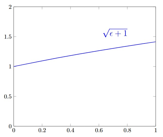
    whose solution is (see figure below)

    \displaystyle x= \sqrt{\epsilon+1}