Month: June 2026

Regularize II

$\displaystyle$

The underlying idea of regularization is to recover the roots that are lost in a singular limit. When some coefficients of a polynomial are multiplied by powers of a small parameter $\epsilon$ , the limiting polynomial obtained by setting $\epsilon=0$ may have fewer roots than the original polynomial. In this situation, some roots have escaped to a different scale and are therefore invisible in the limit.

To recover these missing roots, we introduce a rescaling

$\displaystyle x:=\epsilon^p w$

where the exponent $p$ is chosen so that at least two dominant terms of the polynomial balance each other. Geometrically, this choice is determined from the Newton polygon (or Newton diagram) by examining the exponents of $\epsilon$ . After an additional normalization by a factor $\epsilon^{-m_j}$ , one obtains a new limiting polynomial in the variable $w$ . This reduced polynomial captures the asymptotic behavior of the roots on the corresponding scale and typically restores the correct number of roots.

In this sense, the singularity is not an intrinsic property of the problem but rather the consequence of observing the problem at an inappropriate scale.

As a simple example, consider

$\displaystyle P(x) = x^2 -x+1$

$\displaystyle P_\epsilon(x) =\epsilon x^2-x+1$

Setting $\epsilon=0$ gives

$\displaystyle P_0(x)=-x+1$

which has only one root, although the original polynomial is quadratic and therefore has two roots. To recover the missing root, let

$\displaystyle x:=\epsilon^{-1}w$

Substituting into the polynomial gives

$\displaystyle P_\epsilon(\epsilon^{-1}w) = \epsilon(\epsilon^{-2}w^2)-\epsilon^{-1}w+1 = \epsilon^{-1}(w^2-w+\epsilon)$

Multiplying by $\epsilon$ yields

$\displaystyle w^2-w+\epsilon$

Taking the limit $\epsilon\to0$ gives the regular polynomial

$\displaystyle w^2-w=w(w-1)$

which has two roots. One corresponds to the finite root seen in the original limit, while the second reveals a root located on the larger scale $x=O(\epsilon^{-1})$ . The rescaling has therefore recovered the root that was hidden in the singular limit.

June 25, 2026
Regularize I

We will now present (without justification) a method for regularizing a singular problem involving a polynomial. We want to find the roots of :

$\displaystyle P(x) = x^6 - x^4 - x^3 + 8$

We decide to perturb the above polynomial as follows:

$\displaystyle P_{\epsilon}(x) = \epsilon^2 x^6 - \epsilon x^4 - x^3 + 8$

For $\epsilon = 0$ we have:

$\displaystyle P_{\epsilon= 0}(x) = -x^3 + 8$

This polynomial has three roots. We have a singular problem since the original polynomial has six roots.

We can try to fix the problem using a change of variable:

$\displaystyle x := \epsilon^p w$

$\displaystyle P_{\epsilon}(\epsilon^p w) = \epsilon^2 (\epsilon^p w)^6 - \epsilon (\epsilon^p w)^4 - (\epsilon^p w)^3 + 8$

$\displaystyle = \epsilon^2 (\epsilon^{6p} w^6) - \epsilon (\epsilon^{4p} w^4) - (\epsilon^{3p} w^3) + 8$

$\displaystyle = \epsilon^{6p+2} w^6 - \epsilon^{4p+1} w^4 - \epsilon^{3p} w^3 + 8$

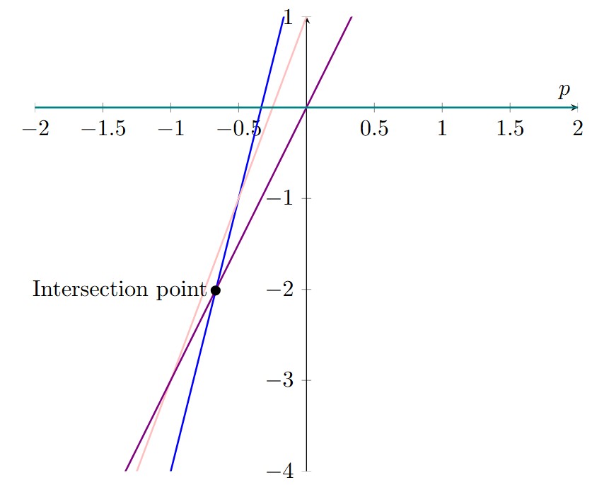
Now we collect the exponents of $\epsilon$ : ( $6p+2, 4p+1$ , $3p, 0$ ) and plot them in a graph as a function of p (see figure below). If we think of the lines on the graph as delimiting a figure in the plane, we can select the vertex of this figure with the largest p value and the smallest f(p) value. In our case, the point corresponding to this criterion is the point of intersection of the lines $6p+2$ and $3p$ . We thus obtain the point of intersection with coordinates ( $-2/3, -2$ ).

We will call the coordinates of the intersection point $p_j$ and $m_j$ respectively.

Now calculate:

$\displaystyle \epsilon^{-m_j} P_{\epsilon}(\epsilon^{p_j} w) = \epsilon^{2} P_{\epsilon}(\epsilon^{-\frac{2}{3}} w)$

$\displaystyle = \epsilon^2 (\epsilon^{6(-\frac{2}{3})+2} w^6 - \epsilon^{4(-\frac{2}{3})+1} w^4 - \epsilon^{3(-\frac{2}{3})} w^3 + 8)$

$\displaystyle = \epsilon^2 (\epsilon^{-2} w^6 - \epsilon^{-\frac{5}{3}} w^4 - \epsilon^{-2} w^3 + 8)$

$\displaystyle = w^6 - \epsilon^{\frac{1}{3}} w^4 - w^3 + 8 \epsilon^2$

This is now a regular problem since the new polynomial:

$\displaystyle P(w) = w^6 - w^3$

has 6 roots.

Using the procedure above we have regularized a singular problem involving a polynomial using the following sequence:

$\displaystyle P(x) \to P_{\epsilon}(x) \to P_{\epsilon}(\epsilon^p w) \to \epsilon^{-m_j} P_{\epsilon}(\epsilon^{p_j} w)$

June 18, 2026
A quintic equation
So far, we’ve introduced the perturbation technique, described regular and irregular problems and presented solutions to simple problems that we could have solved exactly without using perturbative series. We will now consider a problem that cannot be solved exactly. In this way, we hope to illustrate the power of this method.

We want to find a real zero of the following quintic equation:

$\displaystyle x^5 + x = 1$

We will proceed as usual (see previous sections):

$\displaystyle x^5 + \epsilon x = 1$

$\displaystyle (a_0 + a_1\epsilon + a_2 \epsilon^2 + \cdots)^5 + \epsilon (a_0 + a_1\epsilon + a_2 \epsilon^2 + \cdots) = 1$

Solving the unperturbed problem (where $\epsilon = 0$ ) we see that $a_0 = 1$ ( $a_0$ is always the answer to the unperturbed problem). We can use Python to expand the perturbative series and compute the coefficients (see code below). In this example we will calculate up to six coefficients.
```
from sympy import *

# set variables
a1 = Symbol('a1')
a2 = Symbol('a2')
a3 = Symbol('a3')
a4 = Symbol('a4')
a5 = Symbol('a5')
x = Symbol('x') # epsilon

# from the unperturbed problem we know that a0 = 1

# expand the quintic equation
equ = expand ((1 + a1*x + a2*x**2 + a3*x**3 + a4*x**4 + a5*x**5)** 5 + x*(1 + a1*x + a2*x**2 + a3*x**3 + a4*x**4 + a5*x**5))

# get the coefficients separately
equ.coeff(x)

5*a1+1

equ.coeff(x**2)

10*a1**2+a1+5*a2

# solve the system of equations to calculate coefficients
solution = solve([equ.coeff(x),equ.coeff(x**2),equ.coeff(x**3)], (a1, a2, a3))
solution

[(-1/5, -1/25, -1/125)]

solution = solve([equ.coeff(x),equ.coeff(x**2),equ.coeff(x**3),equ.coeff(x**4), equ.coeff(x**5)], (a1, a2, a3, a4, a5))
solution

[(-1/5, -1/25, -1/125, 0, 21/15625)])
```
Therefore (using the results above calculated using Python):

$\displaystyle a_0 = 1$

$\displaystyle a_1 = -\frac{1}{5}$

$\displaystyle a_2 = -\frac{1}{25}$

$\displaystyle a_3 = -\frac{1}{125}$

$\displaystyle a_4 = 0$

$\displaystyle a_5 = \frac{21}{15625}$

We have:

$\displaystyle x(\epsilon) = 1 - \frac{1}{5}\epsilon - \frac{1}{25}\epsilon^2 - \frac{1}{125}\epsilon^3 + 0\cdot\epsilon^4 + \frac{21}{15625}\epsilon^5 + \cdots$

An approximation (fifth-order approximation) of the real solution of $x^5 + x = 1$ is (setting $\epsilon = 1$ ):

$\displaystyle 1 - \frac{1}{5} - \frac{1}{25} - \frac{1}{125} + 0 + \frac{21}{15625} \approx 0.7533$
June 11, 2026
Illustration of a singular problem

Illustration of a singular problem:

$\displaystyle x^2-2x +1 = 0 \quad \text{Problem}$

$\displaystyle \epsilon x^2-2x +1 = 0 \quad \text{Insert }\epsilon$

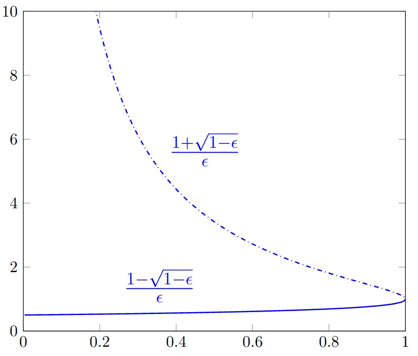
The solutions to the perturbed problem are (see figure below):

$\displaystyle x_1(\epsilon) = \frac{1+ \sqrt{1-\epsilon}}{\epsilon}$

$\displaystyle x_2(\epsilon) = \frac{1- \sqrt{1-\epsilon}}{\epsilon}$

While one of the roots approaches $\frac{1}{2}$ as $\epsilon \to 0$ , the other goes to infinity. This is a manifestation of a singular behaviour. The problems above illustrate the importance of setting $\epsilon$ to a right position.

A solution of the regular problem $x^2-2x +\epsilon = 0$ is $x_1(\epsilon) = 1 - \sqrt{1- \epsilon}$ . We would like to calculate the corresponding perturbative series.
Using:

$\displaystyle (a+b)^n = \sum_{k=0}^{\infty} {n\choose k} a^{n-k}b^{k}$

$\displaystyle = a^n + n a^{n-1}b + \frac{n(n-1)}{2} a^{n-2}b^{2}+...+ \frac{n(n-1)\cdots(n-k+1)}{k!} a^{n-k}b^k +...$

We would like to find the perturbative series corresponding to:

$\displaystyle \sqrt{1-\epsilon} = (1-\epsilon)^{1/2}$

with $a=1$ , $b = -\epsilon$ , $n = \frac{1}{2}$ therefore:

$\displaystyle \sqrt{1-\epsilon} = 1 - \frac{1}{2}\epsilon - \frac{1}{8}\epsilon^2 - ...$

$\displaystyle 1- \sqrt{1-\epsilon} = \frac{1}{2}\epsilon + \frac{1}{8}\epsilon^2 + ...$

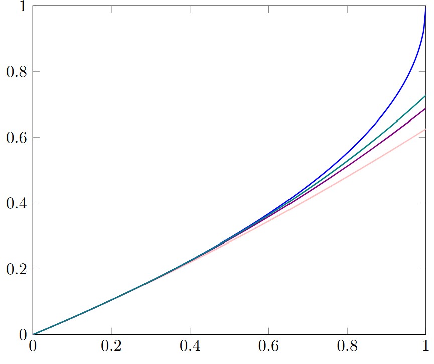
Here are the first series and their corresponding graphs:

$\displaystyle s_2 = \frac{1}{2} \epsilon + \frac{1}{8} \epsilon^2$

$\displaystyle s_3 =\frac{1}{2} \epsilon + \frac{1}{8} \epsilon^2 + \frac{1}{16} \epsilon^3$

$\displaystyle s_4 = \frac{1}{2} \epsilon + \frac{1}{8} \epsilon^2 + \frac{1}{16} \epsilon^3 + \frac{5}{128} \epsilon^4$

June 4, 2026