The Newton Polygon

The construction based on the affine exponent functions (see this post)

\displaystyle L_i(p)=m_ip+\alpha_i

has a simple geometric counterpart known as the Newton polygon. Instead of representing each monomial

\displaystyle \epsilon^{\alpha_i}x^{m_i}

by the affine function L_i(p), we associate it with the point

\displaystyle (m_i,\alpha_i)

in the (m,\alpha) plane. The Newton polygon is defined as the lower convex hull of these points. Its edges contain exactly the information needed to determine the admissible scalings. Indeed, if an edge joins the points

\displaystyle (m_i,\alpha_i) \qquad\text{and}\qquad (m_j,\alpha_j)

its slope is

\displaystyle s=\frac{\alpha_j-\alpha_i}{m_j-m_i}

and the corresponding scaling exponent is

\displaystyle p=-s=-\frac{\alpha_j-\alpha_i}{m_j-m_i}

Thus, each edge of the Newton polygon corresponds to a dominant balance between monomials. The successive edges recover exactly the same admissible scalings as the corners of the lower envelope of the affine functions L_i(p). The Newton polygon therefore provides a dual geometric interpretation of the regularization process. As an illustration, consider the perturbed polynomial (see this post)

\displaystyle P_{\epsilon}(x)=\epsilon^3x^3+x^2+\epsilon x

The corresponding points in the (m,\alpha) plane are

\displaystyle (3,3),\qquad (2,0),\qquad (1,1)

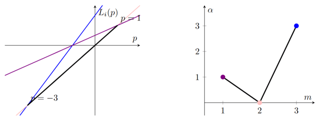
The Newton polygon is the lower convex hull (see figure below)

\displaystyle (1,1)\longrightarrow(2,0)\longrightarrow(3,3)

The first edge has slope

\displaystyle s=\frac{0-1}{2-1}=-1

and therefore gives the scaling

\displaystyle p=1

The second edge has slope

\displaystyle s=\frac{3-0}{3-2}=3

and gives the scaling

\displaystyle p=-3

These two values are exactly the admissible scalings obtained from the intersections of the affine exponent functions

\displaystyle 3p+3,\qquad 2p,\qquad p+1

The left panel of the figure below shows the affine exponent functions and their lower envelope, while the right panel shows the corresponding Newton polygon. The two pictures are dual representations of the same dominant balance structure.
Comments

Leave a comment