After several months of exploring various summation and acceleration methods, it is time to synthesize these tools before we apply them to one of their most important domains: Perturbation Theory.
When a power series 
Summation Methods: Taming Divergence
- Borel and Borel–Écalle: By using the Borel transform, we transform factorially growing coefficients into a convergent series in the Borel plane. The Borel–Écalle framework further allows us to handle singularities via resurgence theory, providing a unique “resummed” value even for non-Borel-summable series.
- Euler and Zeta summation: These methods assign finite values to divergent sums by analytic continuation. While Euler summation is ideal for alternating series, Zeta summation provides a powerful way to handle the infinite sums that frequently appear in quantum vacuum energy calculations.
- Generic summation: Beyond these classical approaches, we have also explored the idea of generic summation, which provides a unifying framework for assigning values to divergent or slowly convergent series.
Acceleration Techniques: Enhancing Convergence
- Shanks Transformation and Padé Approximants: These nonlinear transformations (often related to continued fractions) excel at capturing the behavior of functions beyond their radius of convergence, particularly when poles are present.
- Richardson Extrapolation: A fundamental tool for numerical analysis that cancels out the leading error terms, allowing us to estimate the limit of a sequence Sn with much higher precision from only a few terms.
An important consistency check underlies all these techniques: whenever different summation or acceleration methods apply to the same series, they agree on a common value. This convergence of independent approaches is not accidental, it reflects the fact that these methods capture an underlying analytic object beyond the formal series itself. When they work, they do not merely assign a value: they reveal a coherent extension of the function that the original divergent expansion was hinting at.
 analytic at
  , with Taylor series
 , the Padé approximant of order
 ![[m/n]](https://s0.wp.com/latex.php?latex=%5Bm%2Fn%5D&bg=ffffff&fg=000&s=0&c=20201002) , denoted
, denoted  with
with  and
and  , satisfies
 by modeling singularities (e.g., poles or branch points) through the zeros of
  . This enables analytic continuation into regions where the Taylor series diverges.
 , the diagonal Padé approximants
 ![[n/n]](https://s0.wp.com/latex.php?latex=%5Bn%2Fn%5D&bg=ffffff&fg=000&s=0&c=20201002) often converge to
often converge to  , where
  is the set of poles of
  :
: , with a set of poles
  satisfying
 .
.  be a power series. The denominator
  of the Padé approximant
  is given by Nuttall’s compact form:
 is obtained by satisfying the Padé approximation condition:
  .
. is:
is:


 can be approximated by a sequence of diagonal Padé approximants
  , provided the associated Hankel matrices
  , built from the Taylor coefficients, have nonzero determinants.
 for all
  ), each Padé approximant is uniquely defined.
 :
:


 :
:


 and
and  ) that Padé approximants:
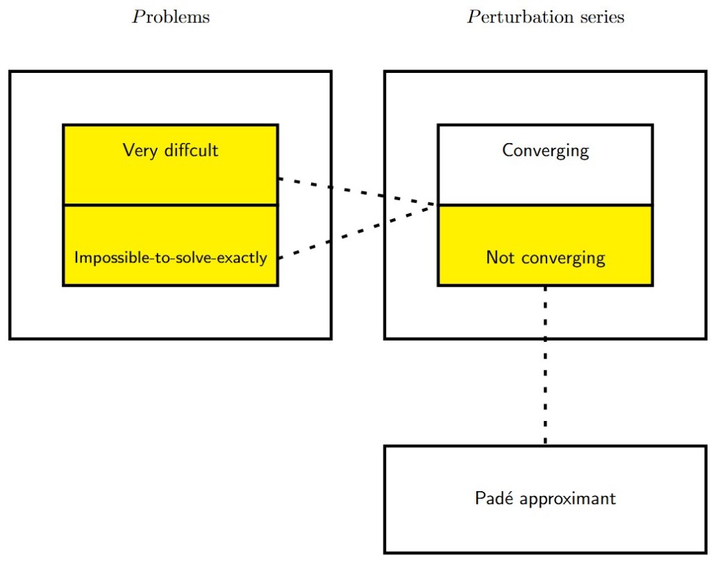

 . This function has two poles at
  and
and  .
.
 approximant is (calculations were made according to the linear systems presented in
 (the total number of poles) we recover the original function since
  . The graphs of the
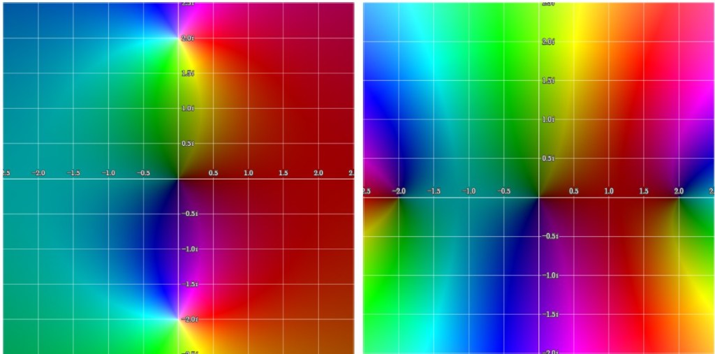


 -plane. The poles at
  and
and  are clearly visible on the left picture. Hue and brightness are used to display phase and magnitude, respectively.

 function. The improvement of the approximation between
  is visible on the figures.
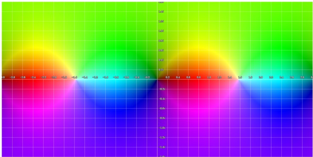


 dont les
  pôles les plus rapprochés de l’origine sont intérieurs à un cercle (C) lui-même intérieur aux pôles suivants, chaque pôle multiple étant compté pour autant de pôles simples qu’il existe d’unités dans son degré de multiplicité, la fraction continue déduite de la ligne horizontale de rang
  , où
, où  est l’affixe du pôle le plus rapproché de l’origine parmi tous ceux qui sont extérieurs au cercle (C). Si tous les pôles ont des modules différents, les fractions continues correspondant aux lignes horizontales représentent toute la fonction ; s’il existe simplement des discontinuités dans l’ensemble linéaire des modules des pôles, les fractions continues correspondant à des lignes horizontales convenablement choisies représentent encore la fonction. Si tous les pôles sont simples, la représentation a lieu dans des cercles d’autant plus grands que la ligne horizontale choisie est plus éloignée dans le Tableau. S’il y a des pôles multiples, il y a stationnement, en ce sens que plusieurs lignes horizontales consécutives représentant la fonction ont le même rayon de convergence. S’il y a enfin un point singulier essentiel, le stationnement se prolonge indéfiniment, aucune des fractions continues considérées ne représente la fonction en dehors du cercle sur la circonférence duquel se trouve le point singulier essentiel le plus rapproché de l’origine.”
 and meromorphic with precisely
  poles (multiplicity counted) in the disk
  . Let D be the domain obtained from
  sufficiently large, there exists a unique rational function
  of type
  , which interpolates
  . Each
  , these poles approach the
  (with multiplicity included) in
  of
of 
 . In particular:


 , with
  , and assume
  at
at  . If
. If  , then the
 ![[n/m]](https://s0.wp.com/latex.php?latex=%5Bn%2Fm%5D&bg=ffffff&fg=000&s=0&c=20201002) Padé approximant of
Padé approximant of  :
:
 .
.

 is bounded near
 is the
  . For example, for
  , the
, the ![[2/2]](https://s0.wp.com/latex.php?latex=%5B2%2F2%5D&bg=ffffff&fg=000&s=0&c=20201002) Padé approximant can be computed, and
Padé approximant can be computed, and  yields a consistent
  ) and at least
  and
and  .
.
 :
:
 , and the error term remains of order
  . Thus,
  satisfies the same Padé condition as
  . By uniqueness of the
