In this post, we provide readers with Python code that enables the derivation of Padé approximants from series coefficients given as input to the algorithm in the form of a coefficient vector. It is also necessary to predefine the degree of the numerator and denominator.
import sympy as sp

def pade_approximation_function(series, m, n):
    """
    Returns the Padé approximation [m/n] in the form of a rational function
    with coefficients simplified as fractions.

    Parameters:
    series : list - Coefficients of the Taylor series (e.g., [1, 0, -1/2, 0, 1/24, ...] for cos(x))
    m : int - Degree of the numerator
    n : int - Degree of the denominator

    Returns:
    sympy.Expr - Rational function P(x)/Q(x) with simplified fractions
    """
    # Check that there are enough terms in the series
    if len(series) < m + n + 1:
        raise ValueError(f"The series must contain at least {m + n + 1} terms for an [m/n] approximation")

    # Convert the series coefficients to simplified fractions
    series = [sp.simplify(sp.Rational(str(c))) for c in series]

    # Symbolic variable
    x = sp.Symbol('x')

    # Coefficients of the numerator P(x) = a0 + a1*x + ... + am*x^m
    a = [sp.Symbol(f'a{i}') for i in range(m + 1)]
    # Coefficients of the denominator Q(x) = 1 + b1*x + ... + bn*x^n (b0 = 1)
    b = [1] + [sp.Symbol(f'b{i}') for i in range(1, n + 1)]

    # Polynomials P(x) and Q(x)
    P = sum(ai * x**i for i, ai in enumerate(a))
    Q = sum(bi * x**i for i, bi in enumerate(b))

    # The truncated series in polynomial form
    S = sum(c * x**i for i, c in enumerate(series))

    # Equation to solve: P(x) - Q(x)*S(x) = 0 up to order m+n
    expr = P - Q * S

    # Extract coefficients of x^0 to x^(m+n) and set the equations to 0
    equations = [sp.expand(expr).coeff(x, k) for k in range(m + n + 1)]

    # Variables to solve for (a0, a1, ..., am, b1, b2, ..., bn)
    unknowns = a + b[1:]

    # Solve the system
    solution = sp.solve(equations, unknowns)

    if not solution:
        raise ValueError("No solution found for this approximation")

    # Simplified coefficients for P(x) and Q(x)
    num_coeffs = [sp.simplify(sp.Rational(str(solution[ai]))) if ai in solution else 0 for ai in a]
    den_coeffs = [1] + [sp.simplify(sp.Rational(str(solution[bi]))) if bi in solution else 0 for bi in b[1:]]

    # Construct the final polynomials
    P_final = sum(coef * x**i for i, coef in enumerate(num_coeffs))
    Q_final = sum(coef * x**i for i, coef in enumerate(den_coeffs))

    # Return the simplified rational function
    return sp.simplify(P_final / Q_final)
Here is the code to compute the Padé(2,2) for 
    # Compute Padé(2,2) for cos(x)
    series = [1, 0, -sp.Rational(1,2), 0, sp.Rational(1,24)]
    m, n = 2, 2
    pade_approx = pade_approximation_function(series, m, n)
    print("Padé(2,2) approximant for cos(x):")
    sp.pprint(pade_approx)


 analytic at
  , with Taylor series
 , the Padé approximant of order
 ![[m/n]](https://s0.wp.com/latex.php?latex=%5Bm%2Fn%5D&bg=ffffff&fg=000&s=0&c=20201002) , denoted
, denoted  with
with  and
and  , satisfies
 by modeling singularities (e.g., poles or branch points) through the zeros of
  . This enables analytic continuation into regions where the Taylor series diverges.
 , the diagonal Padé approximants
 ![[n/n]](https://s0.wp.com/latex.php?latex=%5Bn%2Fn%5D&bg=ffffff&fg=000&s=0&c=20201002) often converge to
often converge to  , where
  is the set of poles of
  :
: , with a set of poles
  satisfying
 .
.  be a power series. The denominator
  of the Padé approximant
  is given by Nuttall’s compact form:
 is obtained by satisfying the Padé approximation condition:
  .
. is:
is:


 can be approximated by a sequence of diagonal Padé approximants
  , provided the associated Hankel matrices
  , built from the Taylor coefficients, have nonzero determinants.
 for all
  ), each Padé approximant is uniquely defined.
 :
:


 :
:


 , the equation becomes:
 as a geometric series. For the ground state
  we write:


 (to recover the initial differential equation) we have:
 and the exact solution is 1.3924.
 is:
is:
 and
and  ) that Padé approximants:
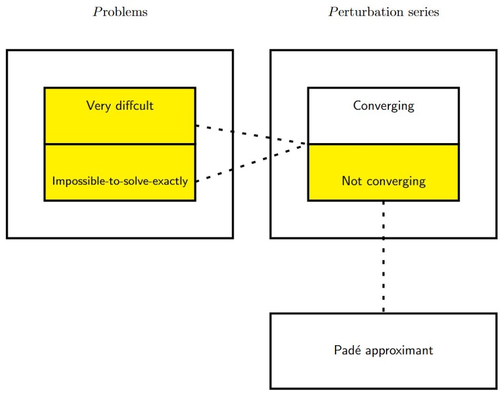

 . This function has two poles at
  and
and  .
.
 approximant is (calculations were made according to the linear systems presented in
 (the total number of poles) we recover the original function since
  . The graphs of the
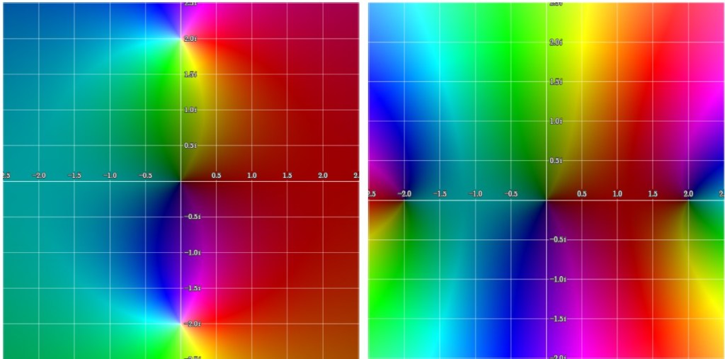


 -plane. The poles at
  and
and  are clearly visible on the left picture. Hue and brightness are used to display phase and magnitude, respectively.

 function. The improvement of the approximation between
  is visible on the figures.
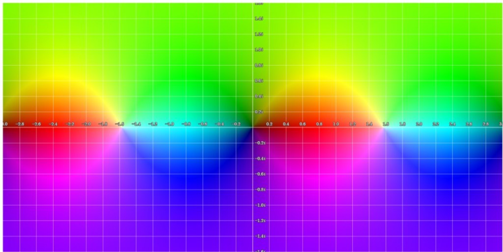


 dont les
  pôles les plus rapprochés de l’origine sont intérieurs à un cercle (C) lui-même intérieur aux pôles suivants, chaque pôle multiple étant compté pour autant de pôles simples qu’il existe d’unités dans son degré de multiplicité, la fraction continue déduite de la ligne horizontale de rang
  , où
, où  est l’affixe du pôle le plus rapproché de l’origine parmi tous ceux qui sont extérieurs au cercle (C). Si tous les pôles ont des modules différents, les fractions continues correspondant aux lignes horizontales représentent toute la fonction ; s’il existe simplement des discontinuités dans l’ensemble linéaire des modules des pôles, les fractions continues correspondant à des lignes horizontales convenablement choisies représentent encore la fonction. Si tous les pôles sont simples, la représentation a lieu dans des cercles d’autant plus grands que la ligne horizontale choisie est plus éloignée dans le Tableau. S’il y a des pôles multiples, il y a stationnement, en ce sens que plusieurs lignes horizontales consécutives représentant la fonction ont le même rayon de convergence. S’il y a enfin un point singulier essentiel, le stationnement se prolonge indéfiniment, aucune des fractions continues considérées ne représente la fonction en dehors du cercle sur la circonférence duquel se trouve le point singulier essentiel le plus rapproché de l’origine.”