Padé approximants of sec(x)

In the previous post we have computed the Padé approximants for the exp(x) function. The approximation was not very impressive compared to the Maclaurin series of exp() since the latter converges for all x. In this post we will have a look at the Padé approximants and Maclaurin series of sec(x).

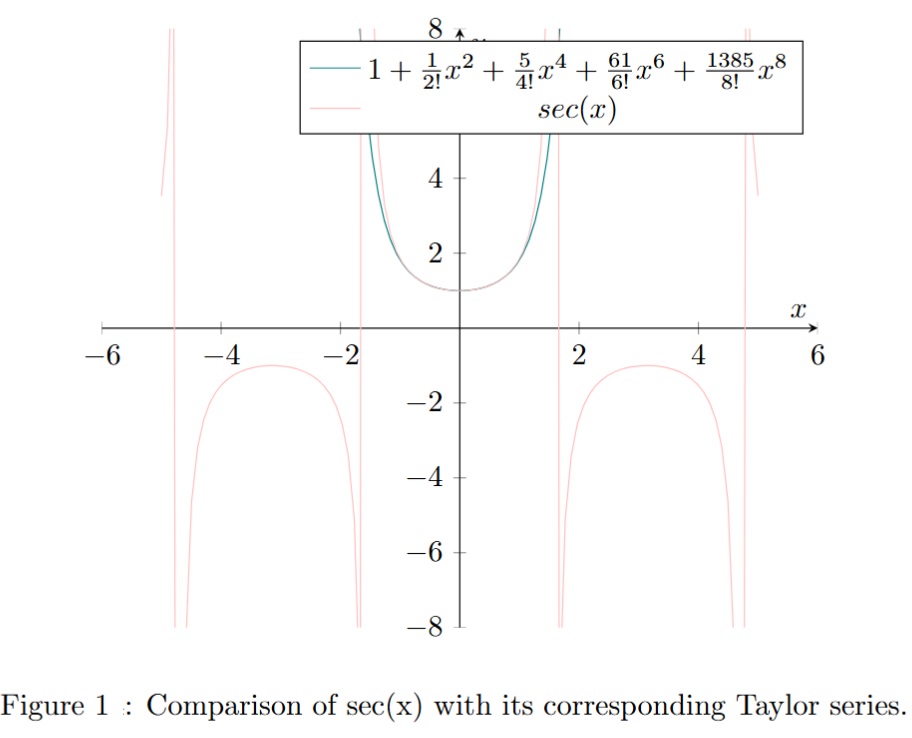
First let’s recall the graph of sec(x) (see figure 1). sec(x) is a function with vertical asymptotes that cannot be approximated globally by a Taylor series. The Maclaurin series of sec(x) is:

\displaystyle sec(x) = 1 + \frac{1}{2!}x^2 + \frac{5}{4!} x^4 + \frac{61}{6!} x^6 + \frac{1385}{8!} x^8 + \cdots
\displaystyle = \sum_{n=0}^{\infty} \frac{E_n}{(2n)!} x^{2n}

Where E_n are so-called Euler numbers:

\displaystyle E_1 = 1, \quad E_2 = 5, \quad E_3 = 61, \quad E_4 = 1385, \quad E_5 = 50521, \quad E_6 = 2702765

We would like to compute the P(4,4) approximant of sec(x). The first step is to have a look at the corresponding Hankel determinant (which is the determinant of the Hankel matrix):

\displaystyle H_{n,m}(f) = \det \left( \begin{array}{cccc} C_{m-n+1} & C_{m-n+2} & \cdots & C_m \\ C_{m-n+2} & C_{m-n+3} & \cdots & C_{m+1} \\ \vdots & \vdots & \ddots & \vdots \\ C_m & C_{m+1} & \cdots & C_{m+n-1} \end{array} \right)

For m = 4 and n = 4 we have:

\displaystyle H_{4,4}(f) = \det \left( \begin{array}{cccc} C_1 & C_2 & C_3 & C_4 \\ C_2 & C_3 & C_4 & C_5 \\ C_3 & C_4 & C_5 & C_6 \\ C_4 & C_5 & C_6 & C_7 \end{array} \right)

and the corresponding Hankel determinant for the P(4,4) of sec(x) is:

\displaystyle H_{4,4}(sec(x)) = \det \left( \begin{array}{cccc} 0 & \frac{1}{2!} & 0 & \frac{5}{4!} \\ \frac{1}{2!} & 0 & \frac{5}{4!} & 0 \\ 0 & \frac{5}{4!} & 0 & \frac{61}{6!} \\ \frac{5}{4!} & 0 & \frac{61}{6!} & 0 \end{array} \right) = 1.08507 \times 10^{-6}

the determinant being not equal to zero implies that we can inverse the Hankel matrix and solve the systems to compute the Padé coefficients of P(4,4) for sec(x) (see post Computing Padé approximants). The inverse of the Hankel matrix is given by:

\displaystyle \left( \begin{array}{cccc} 0 & -81.3333 & 0 & 200 \\ -81.3333 & 0 & 200 & 0 \\ 0 & 200 & 0 & -480 \\ 200 & 0 & -480 & 0 \end{array} \right)

We have to solve this first linear system:

\displaystyle \left( \begin{array}{cccc} 0 & \frac{1}{2!} & 0 & \frac{5}{4!} \\ \frac{1}{2!} & 0 & \frac{5}{4!} & 0 \\ 0 & \frac{5}{4!} & 0 & \frac{61}{6!} \\ \frac{5}{4!} & 0 & \frac{61}{6!} & 0 \end{array} \right) \left( \begin{array}{c} B_4 \\ B_3 \\ B_2 \\ B_1 \end{array} \right) = - \left( \begin{array}{c} C_5 \\ C_6 \\ C_7 \\ C_8 \end{array} \right) = \left( \begin{array}{c} 0 \\ -\frac{61}{6!} \\ 0 \\ -\frac{1385}{8!} \end{array} \right)
\displaystyle \left( \begin{array}{cccc} 0 & \frac{1}{2!} & 0 & \frac{5}{4!} \\ \frac{1}{2!} & 0 & \frac{5}{4!} & 0 \\ 0 & \frac{5}{4!} & 0 & \frac{61}{6!} \\ \frac{5}{4!} & 0 & \frac{61}{6!} & 0 \end{array} \right)^{-1} \left( \begin{array}{c} 0 \\ -\frac{61}{6!} \\ 0 \\ -\frac{1385}{8!} \end{array} \right) = \left( \begin{array}{c} B_4 \\ B_3 \\ B_2 \\ B_1 \end{array} \right)
\displaystyle \left( \begin{array}{cccc} 0 & -81.3333 & 0 & 200 \\ -81.3333 & 0 & 200 & 0 \\ 0 & 200 & 0 & -480 \\ 200 & 0 & -480 & 0 \end{array} \right) \left( \begin{array}{c} 0 \\ -\frac{61}{6!} \\ 0 \\ -\frac{1385}{8!} \end{array} \right) = \left( \begin{array}{c} \frac{104.3191}{5040} \\ 0 \\ -\frac{115}{252} \\ 0 \end{array} \right)

Solving the system above allows us to compute the B_n coefficients (see results below). Now, according to the calculations presented in the post (see Computing Padé approximants), we have to solve the second linear system to compute the A_m coefficients:

\displaystyle \left( \begin{array}{ccccc} C_0 & 0 & 0 & 0 & 0 \\ C_1 & C_0 & 0 & 0 & 0 \\ C_2 & C_1 & C_0 & 0 & 0 \\ C_3 & C_2 & C_1 & C_0 & 0 \\ C_4 & C_3 & C_2 & C_1 & C_0 \end{array} \right) \left( \begin{array}{c} 1 \\ B_1 \\ B_2 \\ B_3 \\ B_4 \end{array} \right) = \left( \begin{array}{c} A_0 \\ A_1 \\ A_2 \\ A_3 \\ A_4 \end{array} \right)
\displaystyle \left( \begin{array}{ccccc} 1 & 0 & 0 & 0 & 0 \\ 0 & 1 & 0 & 0 & 0 \\ \frac{1}{2!} & 0 & 1 & 0 & 0 \\ 0 & \frac{1}{2!} & 0 & 1 & 0 \\ \frac{5}{4!} & 0 & \frac{1}{2!} & 0 & 1 \end{array} \right) \left( \begin{array}{c} 1 \\ 0 \\ -\frac{115}{252} \\ 0 \\ \frac{104.3191}{5040} \end{array} \right) = \left( \begin{array}{c} A_0 \\ A_1 \\ A_2 \\ A_3 \\ A_4 \end{array} \right)
\displaystyle A_0 = 1, \quad A_1 = 0, \quad A_2 = \frac{1}{2!} - \frac{115}{252} = \frac{11}{252}, \quad A_3 = 0, \quad A_4 = \frac{5}{24} - \frac{115}{504} + \frac{104.3191}{5040} = \frac{4.3191}{5040}
\displaystyle B_0 = 1, \quad B_1 = 0, \quad B_2 = -\frac{115}{252}, \quad B_3 = 0, \quad B_4 = \frac{104.3191}{5040}

This implies that for
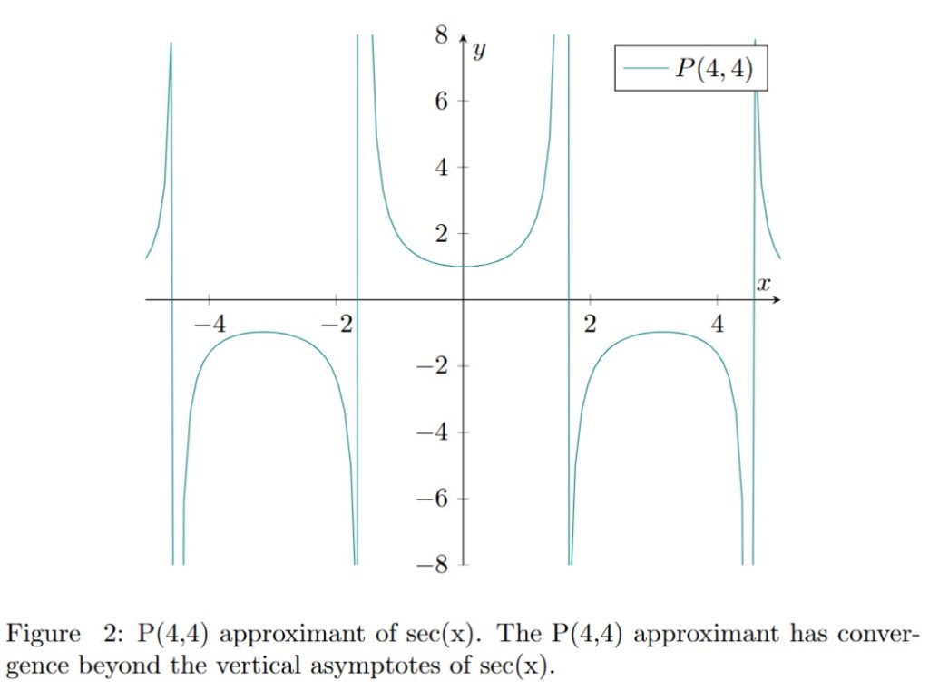
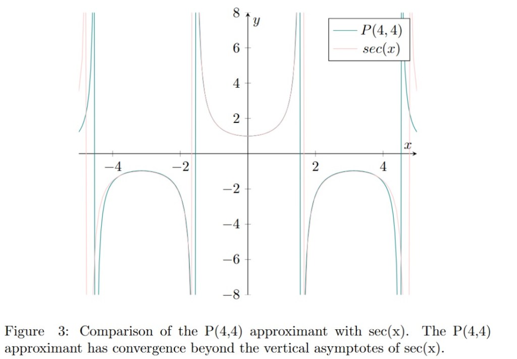
 sec(x):

\displaystyle P(4,4) = \frac{1 + A_2 x^2 + A_4 x^4}{1 + B_2 x^2 + B_4 x^4}
\displaystyle = \frac{1 + \frac{11}{252} x^2 + \frac{4.3191}{5040} x^4}{1 - \frac{115}{252} x^2 + \frac{104.3191}{5040} x^4}

The graph of P(4,4) for sec(x) is presented in figure 2. The graph of sec(x) and its corresponding P(4,4) is presented in figure 3. We can see that the P(4,4) approximant (in green) is approximating the function sec(x) beyond its vertical asymptotes (pink vertical lines) in contrast to the corresponding Taylor series presented in figure 1. Moreover the convergence of P(4,4) is better than the one of the Taylor series.

It is also interesting to note that the ‘information’ needed to construct the Padé approximants of the function sec(x) has been extracted from the truncated Taylor series. Despite this fact, the Padé approximant provides a better approximation of the sec(x) function than the series from which it is derived.

Comments

Leave a comment