In the previous post, we introduced Euler summation. The following are two examples where it fails to produce a finite result.
Consider the divergent series:
Define:
The Euler sum is:
Now consider the divergent series:
Define:
The Euler sum is:
Advantages
Regularization of slowly divergent series:
Euler summation can assign a finite value to some divergent series that oscillate or diverge slowly, such as
where  (series) =
  .
.
Improved convergence:
For many convergent series, Euler transformation accelerates convergence, making it useful for numerical computations.
Analytic continuation link:
It provides a bridge between ordinary summation and more advanced summation methods (e.g. Borel or zeta regularization).
Disadvantages
Limited domain of applicability:
Euler summation fails for series that diverge too rapidly, such as
where (series) =  .
.
Not uniquely defined for all divergent series:
Some series cannot be assigned a finite Euler sum, or the method may yield inconsistent results depending on the transformation order.
Weaker than analytic regularization:
Compared to zeta or Borel summation, Euler’s method handles fewer classes of divergent series and lacks a rigorous analytic continuation framework.


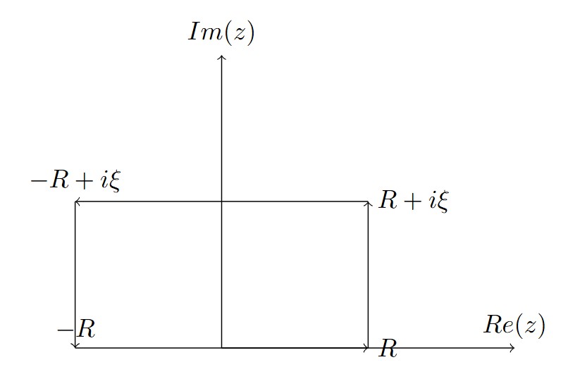
 . This function is an entire function (differentiable in the entire complex plane). Since this function is entire the Cauchy’s integral theorem applies:
 is any closed contour in the complex plane. Let us consider the contour presented in the figure below:
 .
. .
. .
. .
.


 can be written
  :
:


 :
:
 is its own Fourier transform.
 as:
as:

 we should use the analytic continuation of the Zeta function.
 is defined as:
 . If the derivative exists in all points of a region of the complex-plan we say that f(z) is analytic in this region. If the function is analytic inside some circle of convergence
  it can be represented by the Taylor series:
 is the center of the circle
  in
in  the function can be represented by the Taylor series:


 . We would like to show that this function is equivalent to its Fourier transform
 :
:
 :
:


 the analytic continuation of
  has a simple pole at
  lying on the positive real axis. The ordinary Borel integral


 is the exponential integral function. Thus, despite the divergence of the original series and the failure of ordinary Borel summation due to the pole on the integration path, the Borel–Écalle median summation recovers the exact analytic continuation on the positive real axis.


 :
:


 and consider the geometric series:


 and
and  are constants. Equipped with the machine


 is defined as follow:


 converges for
  to
to  therefore:


 is algebraically divergent (the terms blow up like some power of n), then the series:
 . If the limit


