Category: Padé approximants

Padé approximants: Convergence III

For a function $f(z)$ analytic at $z=0$ , with Taylor series

$\displaystyle f(z) = \sum_{k=0}^{\infty} a_k z^k$

valid within its radius of convergence $R$ , the Padé approximant of order $[m/n]$ , denoted $\frac{P_m(z)}{Q_n(z)}$ with $\deg P_m \leq m$ and $\deg Q_n \leq n$ , satisfies

$\displaystyle f(z) - \frac{P_m(z)}{Q_n(z)} = O(z^{m+n+1})$

near $z=0$ . The rational structure of $\frac{P_m(z)}{Q_n(z)}$ allows it to approximate $f(z)$ beyond the disk $|z| < R$ by modeling singularities (e.g., poles or branch points) through the zeros of $Q_n(z)$ . This enables analytic continuation into regions where the Taylor series diverges.

Formally, for a meromorphic function $f(z)$ in a domain $D$ , the diagonal Padé approximants $[n/n]$ often converge to $f(z)$ in $D \setminus S$ , where $S$ is the set of poles of $f$ :

Let $f(z)$ be meromorphic in a domain $D \subseteq \mathbb{C}$ , with a set of poles $S$ of finite total multiplicity. The diagonal Padé approximants $[n/n]$ , defined as rational functions $\frac{P_n(z)}{Q_n(z)}$ satisfying

$\displaystyle f(z) - \frac{P_n(z)}{Q_n(z)} = O(z^{2n+1})$

near $z=0$ , converge uniformly to $f(z)$ on compact subsets of $D \setminus S$ as $n \to \infty$ .

The zeros of $Q_n(z)$ approximate the poles in $S$ , enabling analytic continuation of $f(z)$ beyond the radius of convergence of its Taylor series.

October 23, 2025
Nuttall’s Padé approximant

Let $f(z) = \sum_{k=0}^\infty C_k z^k$ be a power series. The denominator $Q_{n-1}(z)$ of the Padé approximant $P(n, n-1)$ is given by Nuttall’s compact form:

$\displaystyle Q_{n-1}(z) = \frac{ \begin{vmatrix} C_0 & C_1 & C_2 & \cdots & C_{n-1} & C_n \\ C_1 & C_2 & C_3 & \cdots & C_n & C_{n+1} \\ C_2 & C_3 & C_4 & \cdots & C_{n+1} & C_{n+2} \\ \vdots & \vdots & \vdots & \ddots & \vdots & \vdots \\ C_{n-2} & C_{n-1} & C_n & \cdots & C_{2n-3} & C_{2n-2} \\ 1 & z & z^2 & \cdots & z^{n-2} & z^{n-1} \end{vmatrix} }{ \begin{vmatrix} C_0 & C_1 & C_2 & \cdots & C_{n-1} \\ C_1 & C_2 & C_3 & \cdots & C_n \\ C_2 & C_3 & C_4 & \cdots & C_{n+1} \\ \vdots & \vdots & \vdots & \ddots & \vdots \\ C_{n-1} & C_n & C_{n+1} & \cdots & C_{2n-1} \end{vmatrix} }$

The numerator $P_n(z)$ is obtained by satisfying the Padé approximation condition: $f(z) Q_{n-1}(z) - P_n(z) = O(z^{2n})$ .

The compact form of Nuttall’s Padé approximant $P(n, n-1)$ is particularly valuable in numerical analysis and theoretical physics for its efficiency in computing Padé approximants without explicitly solving large linear systems.

By expressing the denominator $Q_{n-1}(z)$ as a ratio of determinants, it provides a direct and elegant method to capture the approximant’s poles, which is crucial for analyzing singularities of functions, especially in Stieltjes series or meromorphic functions.

This formulation simplifies calculations, facilitates the study of convergence properties, and connects Padé approximants to orthogonal polynomials, enabling applications in areas like quantum field theory and asymptotic analysis where rapid computation and singularity detection are essential.

October 16, 2025
Continued fractions II

A well-known continued fraction representation of $exp(x)$ is:

$\displaystyle exp(x) = 1 + \frac{x}{1 - \frac{x}{2 + \frac{x}{3 - \frac{x}{4 + \cdots}}}}$

Using the procedure described in the previous post, we can show that the near-diagonal Padé coefficients presented in this post can be converted to a sequence of truncated fractions corresponding to the continued fraction above (see figures below).

…

$P(m,n)$ $0$ $1$ $2$ $3$

$0$
$\displaystyle 1$

$\displaystyle 1 + x$
…

$1$
$\displaystyle 1 + \cfrac{x}{1 - \cfrac{x}{2}}$

$\displaystyle 1 + \cfrac{x}{1 - \cfrac{x}{2 + \cfrac{x}{3}}}$
…

$2$
$\displaystyle 1 + \cfrac{x}{1 - \cfrac{x}{2 + \cfrac{x}{3 - \cfrac{x}{4}}}}$

$\displaystyle 1 + \cfrac{x}{1 - \cfrac{x}{2 + \cfrac{x}{3 - \cfrac{x}{4 + \cfrac{x}{5}}}}}$
…

$3$ …

… … … … … …

Caption: Padé Approximants P(m,n) for $exp(x)$ expressed as continued fractions.

The relationship between Padé approximants and continued fractions is a profound connection in mathematical analysis, particularly for approximating functions like $exp(x)$ . Padé approximants, which are rational functions that match the Taylor series of a function up to a specified order, can often be expressed as continued fractions. This representation is advantageous because continued fractions can provide better convergence properties for certain functions, especially near singularities. For instance, the near-diagonal Padé approximants for $exp(x)$ , as shown above, can be systematically converted into a sequence of truncated continued fractions, revealing a structured pattern known as the “main Padé sequence.”

A function with a convergent Taylor series around $x = a$ can be approximated by a sequence of diagonal Padé approximants $P(n,n)(x) = \frac{P_n(x)}{Q_n(x)}$ , provided the associated Hankel matrices $H_n$ , built from the Taylor coefficients, have nonzero determinants.

When this “Padé table” is normal (i.e., $\det(H_n) \ne 0$ for all $n$ ), each Padé approximant is uniquely defined.

Under these conditions, one can systematically derive a continued fraction whose successive convergents exactly match the Padé approximants.

This establishes a rigorous connection between the Taylor series, Padé approximation, and continued fraction representation of the function.

October 9, 2025
Continued fractions I

We can use Padé approximants to build a sequence of truncated continued fractions representing a given function. For example using $P(1,1)$ :

$P(1,1) = \frac{A_0 + A_1 x}{1 + B_1 x} = C_0 + C_1 x + C_2 x^2$

Solving the linear systems presented in post Computing Padé approximants sequentially leads to:

$C_1 B_1 = - C_2 \quad \Rightarrow \quad B_1 = -\frac{C_2}{C_1}$

$\begin{pmatrix} C_0 & 0 \\ C_1 & C_0 \end{pmatrix} \begin{pmatrix} 1 \\ B_1 \end{pmatrix} = \begin{pmatrix} A_0 \\ A_1 \end{pmatrix}$

$A_0 = C_0, \quad A_1 = C_1 + C_0 B_1$

Setting $C_0 = 1$ :

$P(1,1) = \frac{1 + (C_1 + B_1) x}{1 + B_1 x}$

$P(1,1) = \frac{1 + (C_1 - \frac{C_2}{C_1}) x}{1 - \frac{C_2}{C_1} x}$

$P(1,1) = \frac{1 + (C_1 - \frac{C_2}{C_1}) x}{1 + (C_1 - \frac{C_2}{C_1}) x - C_1 x}$

$P(1,1) = \frac{1}{1 - \frac{C_1 x}{1 + (C_1 - \frac{C_2}{C_1}) x}}$

$P(1,1) = \frac{1}{1 - \frac{C_1 x}{1 - (\frac{C_2}{C_1} - C_1) x}}$

Now define:

$\frac{b_0}{1 - \frac{b_1 x}{1 - b_2 x}} = \frac{1}{1 - \frac{C_1 x}{1 - \left(\frac{C_2}{C_1} - C_1\right) x}}$

We have:

$b_0 = 1, \quad b_1 = C_1, \quad b_2 = \frac{C_2}{C_1} - C_1, \quad \ldots$

October 2, 2025
Padé approximants: Possible application

The basic idea beyond Padé approximants is to construct a rational fraction whose Taylor series expansion near the origin coincides with that of a given function up to the maximum order. In the previous sections we introduced Padé approximants $P(m,n)$ and a procedure to calculate their coefficients by solving 2 systems of linear equations sequentially (see this post).

We have observed (in particular through the examples concerning $\tan(x)$ and $\sec(x)$ ) that Padé approximants:

Converge beyond the disc of convergence of the entire series

Speed up convergence

Extend the notion of series

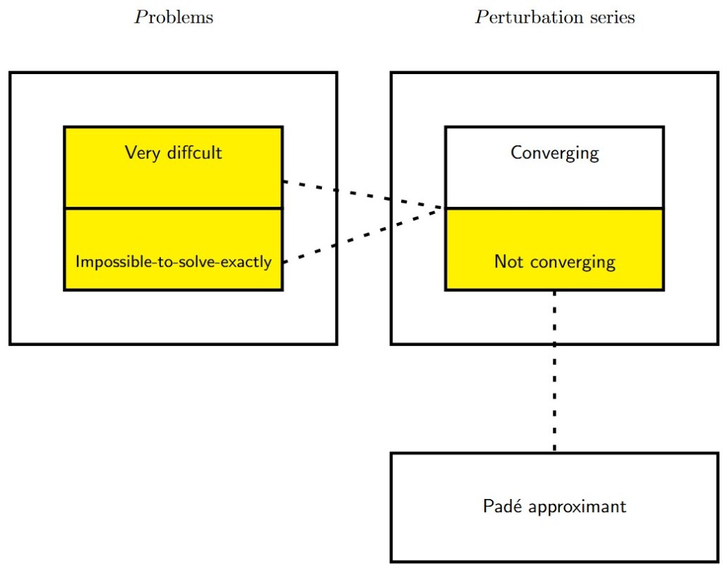
Now, let’s imagine that we want to solve a problem that is very difficult or even impossible to solve exactly (i.e. a specific differential equation, extracting the roots of a polynomial, etc.). We can split the problem into an infinite number of simple problems. This is the principle of perturbation theory (which is in many cases the only way to solve the problem). The result of such a procedure is a geometric series (we will see this later). In a very large number of cases, this series does not converge. In these cases, we can use Padé approximants to ‘extract’ the information contained in the series and finally obtain a convergent rational function (as illustrated in the case of the functions $\tan(x)$ and $\sec(x)$ ).

The figure below presents schematically a potential application of Padé approximants in this context.

September 11, 2025
Padé approximants: Convergence examples

We will first illustrate the Montessus’s theorem with the function:

$\displaystyle f(z) = \frac{z}{4 + z^2} = \frac{z}{(z - 2i)(z + 2i)}$

where $z \in \mathbb{C}$ . This function has two poles at $z = 2i$ and $z = -2i$ .

The corresponding Maclaurin series is:

$\displaystyle \frac{1}{4}z - \frac{1}{16}z^3 + \frac{1}{64}z^5 - \frac{1}{256}z^7 + \frac{1}{1024}z^9 + \mathcal{O}(z^{11})$

The corresponding $P(2,2)$ approximant is (calculations were made according to the linear systems presented in this post):

$\displaystyle P(2,2) = \frac{z}{4 + z^2}$

We see that, in this case, if we set $n = 2$ (the total number of poles) we recover the original function since $P(2,2) = f(z)$ . The graphs of the $f(z)$ , $P(2,2)$ and the corresponding Maclaurin series are presented in the figure below.

Left, graph of

$\displaystyle \frac{z}{4 + z^2}$

and its corresponding $P(2,2)$ . Right, graph of the Maclaurin series

$\displaystyle \frac{1}{4}z - \frac{1}{16}z^3$

in the complex $\mathbb{C}$ -plane. The poles at $-2i$ and $2i$ are clearly visible on the left picture. Hue and brightness are used to display phase and magnitude, respectively.

The Montessus’s theorem is also illustrated in the figures below for the function tan(z).

$\displaystyle P(2,2) = \frac{z}{1 - \frac{1}{3}z^2}$

and

$\displaystyle P(4,2) = \frac{z + \frac{1}{3}z^2}{1 - \frac{6}{15}z^2}$

of the $\tan(z)$ function. The improvement of the approximation between $P(2,2)$ and $P(4,2)$ is visible on the figures.

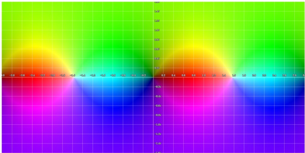
Graph of tan(z):

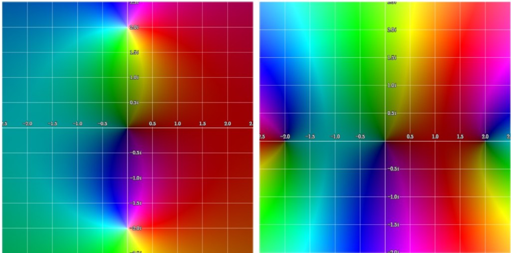
Graphs of the P(2,2) (left) and P(4,2) (right) of tan(z):

Pictures were produced using: Samuel Jinglian, 2018. “Complex Function Plotter.” https://samuelj.li/complex-function-plotter/.

September 4, 2025
Padé approximants: Convergence II
In the previous post we gave a modern definition of Montessus’s theorem. Here is the original formulation from R. De Montessus (1902):

“Il ressort de ces considérations qu’étant donnée une série de Taylor représentant une fonction $f(x)$ dont les $p$ pôles les plus rapprochés de l’origine sont intérieurs à un cercle (C) lui-même intérieur aux pôles suivants, chaque pôle multiple étant compté pour autant de pôles simples qu’il existe d’unités dans son degré de multiplicité, la fraction continue déduite de la ligne horizontale de rang $p$ du Tableau de M. Padé, ce tableau étant composé de réduites normales, représente la fonction $f(x)$ dans un cercle de rayon $\displaystyle \lvert \alpha_{p+1} \lvert$ , où $\alpha_{p+1}$ est l’affixe du pôle le plus rapproché de l’origine parmi tous ceux qui sont extérieurs au cercle (C). Si tous les pôles ont des modules différents, les fractions continues correspondant aux lignes horizontales représentent toute la fonction ; s’il existe simplement des discontinuités dans l’ensemble linéaire des modules des pôles, les fractions continues correspondant à des lignes horizontales convenablement choisies représentent encore la fonction. Si tous les pôles sont simples, la représentation a lieu dans des cercles d’autant plus grands que la ligne horizontale choisie est plus éloignée dans le Tableau. S’il y a des pôles multiples, il y a stationnement, en ce sens que plusieurs lignes horizontales consécutives représentant la fonction ont le même rayon de convergence. S’il y a enfin un point singulier essentiel, le stationnement se prolonge indéfiniment, aucune des fractions continues considérées ne représente la fonction en dehors du cercle sur la circonférence duquel se trouve le point singulier essentiel le plus rapproché de l’origine.”

References:
- R. De Montessus, “Sur les fractions continues algébriques”, Bulletin de la S. M. F., tome 30 (1902), p. 28-36.
- E. B. Saff, “An extension of Montessus de Ballore’s theorem on the convergence of interpolating rational functions”, Journal of Approximation Theory, vol 6, No. 1, July 1972.
August 28, 2025
Padé approximants: Convergence I

For row sequences on the Padé table, Montessus’s theorem (1902) proves convergence for functions meromorphic on a disk. Before giving the statement of the theorem, we would like to remind the reader of a few definitions:

Holomorphic function: A holomorphic function is a complex-valued function of one or more complex variables that is complex differentiable in a neighborhood of each point in a given domain.

Analytic function: An analytic function is a function that is locally given by a convergent power series.

Meromorphic function: A meromorphic function on an open subset D of the complex $\mathbb{C}$ -plane is a function that is holomorphic on all of D except for a set of isolated points. These points are called the ‘poles’ of the function.

Here is the Montessus’s theorem as stated by E. B. Saff in 1972:

Let $f(z)$ be analytic at $z = 0$ and meromorphic with precisely $\nu$ poles (multiplicity counted) in the disk $|z| < \tau$ . Let D be the domain obtained from $|z| < \tau$ by deleting the $\nu$ poles of $f(z)$ . Then, for all $m$ sufficiently large, there exists a unique rational function $R_{m, \nu}$ of type $(m, \nu)$ , which interpolates $f(z)$ in the point $z = 0$ considered of multiplicity $m+\nu+1$ . Each $R_{m, \nu}$ has precisely $\nu$ finite poles and, as $m \to \infty$ , these poles approach the $\nu$ poles of $f(z)$ in $|z| < \tau$ . The sequence $R_{m, \nu}$ converges in D to $f(z)$ , uniformly on any compact subset of D.

Alternative formulation:

Let $f(z)$ be meromorphic in $|z| < \tau$ , analytic at $z = 0$ , and with a total of $\nu$ poles $\zeta_1, \zeta_2, \dots, \zeta_{\nu}$ (with multiplicity included) in $|z| < \tau$ . Then, as $m \to \infty$ , the Padé approximants $P(m,\nu)$ of $f$ converge on:

$\displaystyle S_f := \{ z \in \mathbb{C} \mid |z| < \tau \} \setminus \{ \zeta_1, \zeta_2, \dots, \zeta_\nu \}$

to $f$ , uniformly on every compact subset K of $S_f$ . In particular:

$\displaystyle P(m,\nu)(z) \to f(z)$

The Padé table is represented as follows:

$n=0$ $n=1$ $n=2$ $\dots$ $n=\nu$ $\dots$

$m=0$ $P(0,0)$ $P(0,1)$ $P(0,2)$ $\dots$ $\boxed{P(0,\nu)}$ $\dots$

$m=1$ $P(1,0)$ $P(1,1)$ $P(1,2)$ $\dots$ $\boxed{P(1,\nu)}$ $\dots$

$m=2$ $P(2,0)$ $P(2,1)$ $P(2,2)$ $\dots$ $\boxed{P(2,\nu)}$ $\dots$

$\dots$ $\dots$ $\dots$ $\dots$ $\dots$

$m \to \infty$ $\dots$ $\dots$ $\dots$ $\boxed{P(m,\nu)}$ $\dots$

The Montessus’s theorem is crucial in approximation theory as it ensures the uniform convergence of Padé approximants for meromorphic functions, enhancing the accuracy of rational approximations.

August 21, 2025
Two properties of Padé Approximants

Property 1

Let $g(x) = \frac{1}{f(x)}$ , with $f(0) \neq 0$ , and assume $f$ is at least $C^{m+n}$ at $x = 0$ . If $P(m,n)_f = \frac{P(x)}{Q(x)}$ , then the $[n/m]$ Padé approximant of $g(x)$ :

$\displaystyle P(n,m)_g = \frac{Q(x)}{P(x)},$

provided $P(0) \neq 0$ .

Proof: Given $P(m,n)_f = \frac{P(x)}{Q(x)}$ , we have:

$\displaystyle f(x) Q(x) - P(x) = \epsilon(x) x^{m+n+1}.$

Since $g(x) = \frac{1}{f(x)}$ , consider:

$\displaystyle g(x) P(x) - Q(x) = \frac{1}{f(x)} P(x) - Q(x) = \frac{P(x) - f(x) Q(x)}{f(x)} = -\frac{\epsilon(x) x^{m+n+1}}{f(x)}.$

Since $f(0) \neq 0$ , $\frac{1}{f(x)}$ is bounded near $x = 0$ , and:

$\displaystyle g(x) P(x) - Q(x) = O(x^{m+n+1}),$

indicating that $\frac{Q(x)}{P(x)}$ is the $[n/m]$ Padé approximant of $g(x)$ , as it matches the Taylor series of $g(x)$ up to $x^{m+n}$ . For example, for $f(x) = \sqrt{1+x}$ , the $[2/2]$ Padé approximant can be computed, and $g(x) = \frac{1}{\sqrt{1+x}}$ yields a consistent $[2/2]$ approximant by taking the reciprocal.

Property 2

If $f$ is even ( $f(x) = f(-x)$ ) and at least $C^{m+n}$ , and the $[m/n]$ Padé approximant exists and is unique (guaranteed if the Hankel determinant is non-zero), then $P(m,n)_f = \frac{P(x)}{Q(x)}$ is even, i.e., $P(x) = P(-x)$ and $Q(x) = Q(-x)$ .

Proof: Since $f(x) = f(-x)$ , the Taylor series of $f$ contains only even powers. For $P(m,n)_f = \frac{P(x)}{Q(x)}$ , we have:

$\displaystyle f(x) Q(x) - P(x) = O(x^{m+n+1}).$

Evaluate at $-x$ :

$\displaystyle f(-x) Q(-x) - P(-x) = f(x) Q(-x) - P(-x) = O(x^{m+n+1}),$

since $f(-x) = f(x)$ , and the error term remains of order $x^{m+n+1}$ . Thus, $\frac{P(-x)}{Q(-x)}$ satisfies the same Padé condition as $\frac{P(x)}{Q(x)}$ . By uniqueness of the $[m/n]$ approximant (assuming non-zero Hankel determinant), we conclude:

$\displaystyle P(x) = P(-x), \quad Q(x) = Q(-x).$

August 14, 2025
Padé approximant of 1/(1-x)

In this post we will have a look at the Padé approximants of $\frac{1}{1-x}$ . The Maclaurin series of $\frac{1}{1-x}$ is:

$\displaystyle 1 + x + x^2 + x^3 + x^4 + x^5 + \cdots$

which converges for $x \in ]-1,1[$ . We can calculate the corresponding $P(1,1)$

$\displaystyle \frac{A_0 + A_1 x}{1 + B_1 x} = 1 + x + x^2 + \cdots$

$\displaystyle = (1 + B_1 x)(1 + x + x^2 + \cdots)$

$\displaystyle = 1 + x + x^2 + \cdots + B_1 x + B_1 x^2 + B_1 x^3 + \cdots$

$\displaystyle = 1 + (1 + B_1) x + (1 + B_1) x^2 + (1 + B_1) x^3 + \cdots$

Keeping only degrees up to 2:

$\displaystyle = 1 + (1 + B_1) x + (1 + B_1) x^2$

This implies:

$\displaystyle A_0 = 1$

$\displaystyle A_1 = 1 + B_1$

$\displaystyle 1 + B_1 = 0$

Therefore, $A_0 = 1$ , $A_1 = 0$ and $B_1 = -1$ and the $P(1,1)$ is:

$\displaystyle \boxed{P(1,1)(x) = \frac{1}{1-x}}$

This is an exceptional result since the Padé approximant $P(1,1)$ is equal to the function it is supposed to approximate. This result is very attractive since it suggests a way to solve very hard problems using series up to some terms. Then using Padé approximation we may hope to recover the exact solution (or at least a sufficient approximation for a specific application).

Let’s imagine that we would like to solve the following differential equation:

$\displaystyle y' = y^2 \text{ with initial condition } y(0) = 1$

This differential equation can be solved exactly since it is separable. The solution is $y(x) = \frac{1}{1-x}$ . Let’s pretend for a moment that solving this equation is a very difficult problem because we don’t know how to solve separable differential equations.

A possible approach is to consider a solution of the form:

$\displaystyle y(x) = a_0 + a_1 x + a_2 x^2 + a_3 x^3 + \cdots$

Then we have:

$\displaystyle y(x)' = a_1 + 2 a_2 x + 3 a_3 x^2 + \cdots$

$\displaystyle y(x)^2 = (a_0 + a_1 x + a_2 x^2 + \cdots)^2$

$\displaystyle = a_0^2 + a_0 a_1 x + a_0 a_2 x^2 + \cdots$

$\displaystyle + a_0 a_1 x + a_1^2 x^2 + \cdots$

$\displaystyle + a_2 a_0 x^2 + \cdots$

$\displaystyle = a_0^2 + 2 a_0 a_1 x + (a_1^2 + 2 a_0 a_2) x^2 + \cdots$

We can write the differential equation keeping only terms up to two:

$\displaystyle y(x)' = y(x)^2$

$\displaystyle a_1 + 2 a_2 x + 3 a_3 x^2 = a_0^2 + 2 a_0 a_1 x + (a_1^2 + 2 a_0 a_2) x^2$

we obtain:

$\displaystyle a_1 = a_0^2$

$\displaystyle 2 a_2 = 2 a_0 a_1$

$\displaystyle 3 a_3 = a_1^2 + 2 a_0 a_2$

Setting $a_0 = 1$ (since $y(0) = 1$ ) implies $a_1 = a_2 = a_3 = 1$ . An approximation of the solution to the differential equation is therefore:

$\displaystyle 1 + x + x^2 + x^3$

As presented above, the corresponding $P(1,1) = \frac{1}{1-x}$ which is the exact solution to the differential equation. In fact, the diagonal sequence of Padé approximants ( $P(1,1)$ , $P(2,2)$ , … $P(n,n)$ ) recovers $\frac{1}{1-x}$ . This is, of course, a special case.

So, for this differential equation, we have the following pattern:

August 7, 2025