Month: September 2025

Python code for Padé approximants

In this post, we provide readers with Python code that enables the derivation of Padé approximants from series coefficients given as input to the algorithm in the form of a coefficient vector. It is also necessary to predefine the degree of the numerator and denominator.

import sympy as sp

def pade_approximation_function(series, m, n):
    """
    Returns the Padé approximation [m/n] in the form of a rational function
    with coefficients simplified as fractions.
    
    Parameters:
    series : list - Coefficients of the Taylor series (e.g., [1, 0, -1/2, 0, 1/24, ...] for cos(x))
    m : int - Degree of the numerator
    n : int - Degree of the denominator
    
    Returns:
    sympy.Expr - Rational function P(x)/Q(x) with simplified fractions
    """
    # Check that there are enough terms in the series
    if len(series) < m + n + 1:
        raise ValueError(f"The series must contain at least {m + n + 1} terms for an [m/n] approximation")

    # Convert the series coefficients to simplified fractions
    series = [sp.simplify(sp.Rational(str(c))) for c in series]
    
    # Symbolic variable
    x = sp.Symbol('x')
    
    # Coefficients of the numerator P(x) = a0 + a1*x + ... + am*x^m
    a = [sp.Symbol(f'a{i}') for i in range(m + 1)]
    # Coefficients of the denominator Q(x) = 1 + b1*x + ... + bn*x^n (b0 = 1)
    b = [1] + [sp.Symbol(f'b{i}') for i in range(1, n + 1)]
    
    # Polynomials P(x) and Q(x)
    P = sum(ai * x**i for i, ai in enumerate(a))
    Q = sum(bi * x**i for i, bi in enumerate(b))
    
    # The truncated series in polynomial form
    S = sum(c * x**i for i, c in enumerate(series))
    
    # Equation to solve: P(x) - Q(x)*S(x) = 0 up to order m+n
    expr = P - Q * S
    
    # Extract coefficients of x^0 to x^(m+n) and set the equations to 0
    equations = [sp.expand(expr).coeff(x, k) for k in range(m + n + 1)]
    
    # Variables to solve for (a0, a1, ..., am, b1, b2, ..., bn)
    unknowns = a + b[1:]
    
    # Solve the system
    solution = sp.solve(equations, unknowns)
    
    if not solution:
        raise ValueError("No solution found for this approximation")
    
    # Simplified coefficients for P(x) and Q(x)
    num_coeffs = [sp.simplify(sp.Rational(str(solution[ai]))) if ai in solution else 0 for ai in a]
    den_coeffs = [1] + [sp.simplify(sp.Rational(str(solution[bi]))) if bi in solution else 0 for bi in b[1:]]
    
    # Construct the final polynomials
    P_final = sum(coef * x**i for i, coef in enumerate(num_coeffs))
    Q_final = sum(coef * x**i for i, coef in enumerate(den_coeffs))
    
    # Return the simplified rational function
    return sp.simplify(P_final / Q_final)

Here is the code to compute the Padé(2,2) for $\cos(x)$

    # Compute Padé(2,2) for cos(x)
    series = [1, 0, -sp.Rational(1,2), 0, sp.Rational(1,24)]
    m, n = 2, 2
    pade_approx = pade_approximation_function(series, m, n)
    print("Padé(2,2) approximant for cos(x):")
    sp.pprint(pade_approx)

September 25, 2025

Anharmonic oscillator I

We would like to illustrate the use of Padé approximants in the context of the anharmonic oscillator. A harmonic oscillator is an oscillating system that experiences a restoring force. Anharmonicity is the deviation of a system from being a harmonic oscillator. The anharmonic oscillator is described by the following differential equation:

$\displaystyle \left(-\frac{d^2}{dx^2} + x^2 + x^4\right) \phi(x) = E_n \phi(x)$

This differential equation is very hard to solve exactly. In order to obtain an approximate solution, we can use perturbation theory. By inserting a small dimensionless parameter $\epsilon$ , the equation becomes:

$\displaystyle \left(-\frac{d^2}{dx^2} + x^2 + \epsilon x^4\right) \phi(x) = E_n(\epsilon) \phi(x)$

If we are interested in the energy levels, the basic idea is to write $E_n(\epsilon)$ as a geometric series. For the ground state $E_0$ we write:

$\displaystyle E_0(\epsilon) = \sum_{n=0}^{\infty} E_{0,n} \epsilon^n$

The solution is a divergent perturbation series (C.M. Bender and T.T. Wu, Phys. Rev. 184, 1969):

$\displaystyle E_0(\epsilon) = \frac{1}{2} + \frac{3}{4}\epsilon - \frac{21}{8}\epsilon^2 + \frac{333}{16}\epsilon^3 + \mathcal{O}(\epsilon^4)$

Let’s calculate the $P(1,1)$ approximant of $E_0$ using the techniques presented in post Computing Padé approximants:

$\displaystyle P(1,1) = \frac{A_0 + A_1 \epsilon}{1 + B_1 \epsilon} = C_0 + C_1 \epsilon + C_2 \epsilon^2$

Solving the linear systems for computing Padé approximants sequentially leads to:

$\displaystyle C_1 B_1 = - C_2 \implies B_1 = -\frac{C_2}{C_1}$

$\displaystyle \frac{3}{4} B_1 = \frac{21}{8} \implies B_1 = \frac{84}{24} = \frac{7}{2}$

$\displaystyle \begin{pmatrix} C_0 & 0 \\ C_1 & C_0 \\ \end{pmatrix} \begin{pmatrix} 1 \\ B_1 \end{pmatrix} = \begin{pmatrix} A_0 \\ A_1 \end{pmatrix}$

$\displaystyle \begin{pmatrix} \frac{1}{2} & 0 \\ \frac{3}{4} & \frac{1}{2} \\ \end{pmatrix} \begin{pmatrix} 1 \\ \frac{7}{2} \end{pmatrix} = \begin{pmatrix} \frac{1}{2} \\ \frac{3}{4} + \frac{7}{4} \end{pmatrix}$

$\displaystyle P(1,1)_{E_0} = \frac{\frac{1}{2} + \left(\frac{3}{4} + \frac{7}{4}\right)\epsilon}{1 + \frac{7}{2}\epsilon}$

Setting $\epsilon = 1$ (to recover the initial differential equation) we have:

$\displaystyle P(1,1)_{E_0} = \frac{\frac{1}{2} + \frac{3}{4} + \frac{7}{4}}{1 + \frac{7}{2}} = 0.6666$

The $P(4,4)_{E_0} = 1.3838$ and the exact solution is 1.3924.

The relative error (definition here) of the approximant $P(4,4)_{E_0}$ is:

$\displaystyle \text{Relative error} = \frac{1.3838 - 1.3924}{1.3924} = -0.0062$

It’s therefore interesting to note that in order to solve a very difficult differential equation, we can use perturbation theory. In the case of the anharmonic oscillator, the perturbative series is divergent. Using Padé approximants, we can make use of a divergent perturbative series and approximate the exact answer arbitrarily.

September 18, 2025
Padé approximants: Possible application

The basic idea beyond Padé approximants is to construct a rational fraction whose Taylor series expansion near the origin coincides with that of a given function up to the maximum order. In the previous sections we introduced Padé approximants $P(m,n)$ and a procedure to calculate their coefficients by solving 2 systems of linear equations sequentially (see this post).

We have observed (in particular through the examples concerning $\tan(x)$ and $\sec(x)$ ) that Padé approximants:

Converge beyond the disc of convergence of the entire series

Speed up convergence

Extend the notion of series

Now, let’s imagine that we want to solve a problem that is very difficult or even impossible to solve exactly (i.e. a specific differential equation, extracting the roots of a polynomial, etc.). We can split the problem into an infinite number of simple problems. This is the principle of perturbation theory (which is in many cases the only way to solve the problem). The result of such a procedure is a geometric series (we will see this later). In a very large number of cases, this series does not converge. In these cases, we can use Padé approximants to ‘extract’ the information contained in the series and finally obtain a convergent rational function (as illustrated in the case of the functions $\tan(x)$ and $\sec(x)$ ).

The figure below presents schematically a potential application of Padé approximants in this context.

September 11, 2025
Padé approximants: Convergence examples

We will first illustrate the Montessus’s theorem with the function:

$\displaystyle f(z) = \frac{z}{4 + z^2} = \frac{z}{(z - 2i)(z + 2i)}$

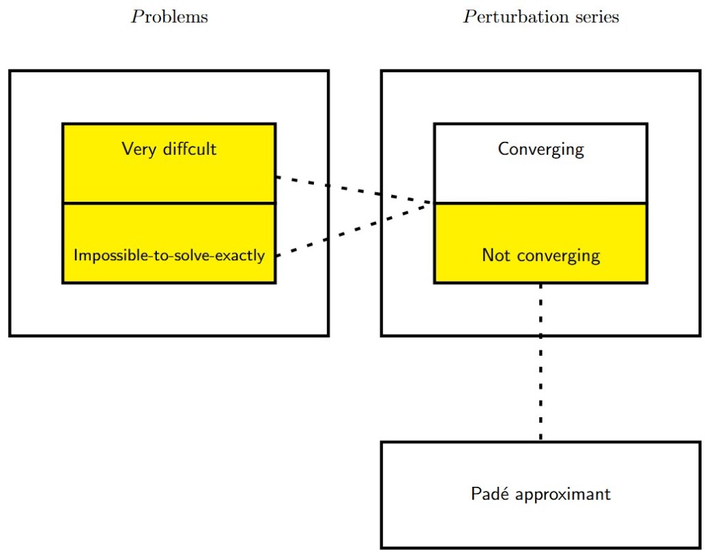
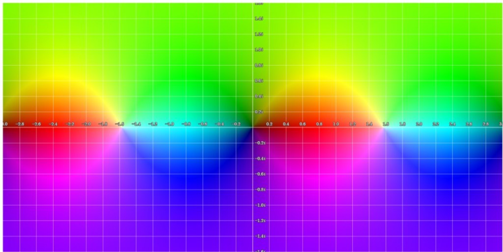
where $z \in \mathbb{C}$ . This function has two poles at $z = 2i$ and $z = -2i$ .

The corresponding Maclaurin series is:

$\displaystyle \frac{1}{4}z - \frac{1}{16}z^3 + \frac{1}{64}z^5 - \frac{1}{256}z^7 + \frac{1}{1024}z^9 + \mathcal{O}(z^{11})$

The corresponding $P(2,2)$ approximant is (calculations were made according to the linear systems presented in this post):

$\displaystyle P(2,2) = \frac{z}{4 + z^2}$

We see that, in this case, if we set $n = 2$ (the total number of poles) we recover the original function since $P(2,2) = f(z)$ . The graphs of the $f(z)$ , $P(2,2)$ and the corresponding Maclaurin series are presented in the figure below.

Left, graph of

$\displaystyle \frac{z}{4 + z^2}$

and its corresponding $P(2,2)$ . Right, graph of the Maclaurin series

$\displaystyle \frac{1}{4}z - \frac{1}{16}z^3$

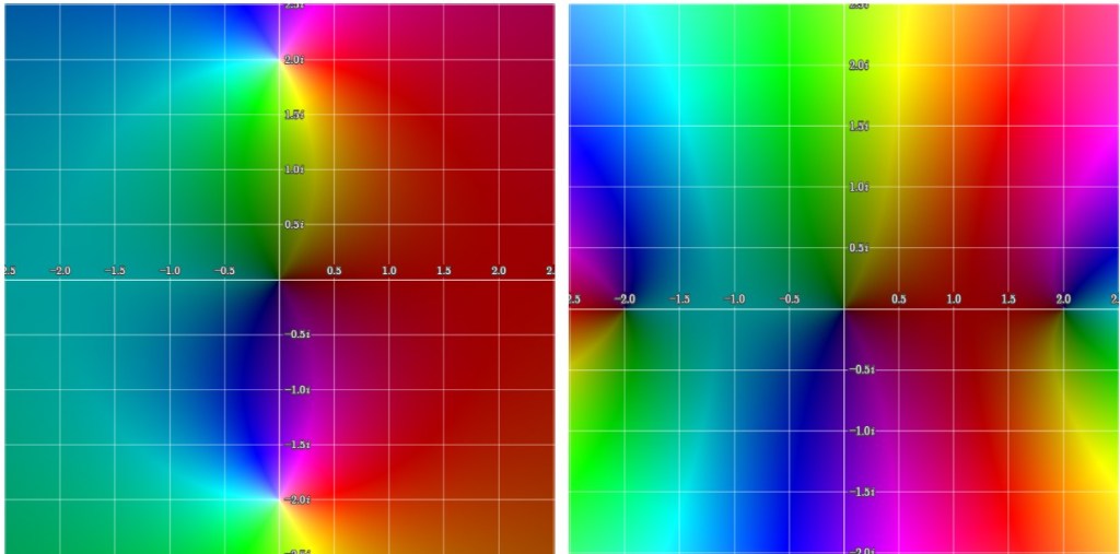
in the complex $\mathbb{C}$ -plane. The poles at $-2i$ and $2i$ are clearly visible on the left picture. Hue and brightness are used to display phase and magnitude, respectively.

The Montessus’s theorem is also illustrated in the figures below for the function tan(z).

$\displaystyle P(2,2) = \frac{z}{1 - \frac{1}{3}z^2}$

and

$\displaystyle P(4,2) = \frac{z + \frac{1}{3}z^2}{1 - \frac{6}{15}z^2}$

of the $\tan(z)$ function. The improvement of the approximation between $P(2,2)$ and $P(4,2)$ is visible on the figures.

Graph of tan(z):

Graphs of the P(2,2) (left) and P(4,2) (right) of tan(z):

Pictures were produced using: Samuel Jinglian, 2018. “Complex Function Plotter.” https://samuelj.li/complex-function-plotter/.

September 4, 2025