Month: July 2025

Padé approximants of sqrt(1+x) and 1/sqrt(1+x)

In this post we will have a look at the Padé approximants of $\sqrt{1+x}$ and $\frac{1}{\sqrt{1+x}}$ . The Maclaurin series of $\sqrt{1+x}$ is:

$\displaystyle 1+ \frac{1}{2}x - \frac{1}{8} x^2 + \frac{1}{16}x^3 - \frac{5}{128} x^4 + \frac{7}{256}x^5 + \dots$

The MacLaurin series of $\frac{1}{\sqrt{1+x}}$ is:

$\displaystyle 1 - \frac{1}{2}x + \frac{3}{8}x^2 - \frac{5}{16}x^3 + \frac{35}{128}x^4 + \dots$

According to the section concerning the calculation of Padé approximants using a matrix notation (see post Computing Padé approximants, we have to solve two linear systems sequentially. For $\sqrt{1+x}$ we therefore have to first solve:

$\displaystyle \begin{pmatrix} C_1 & C_2 \\ C_2 & C_3 \end{pmatrix} \begin{pmatrix} B_2 \\ B_1 \end{pmatrix} = -\begin{pmatrix} C_3 \\ C_4 \end{pmatrix}$

$\displaystyle \begin{pmatrix} \frac{1}{2} & -\frac{1}{8} \\ -\frac{1}{8} & \frac{1}{16} \end{pmatrix} \begin{pmatrix} B_2 \\ B_1 \end{pmatrix} = \begin{pmatrix} -\frac{1}{16} \\ \frac{5}{128} \end{pmatrix}$

$\displaystyle \begin{pmatrix} B_2 \\ B_1 \end{pmatrix} = \begin{pmatrix} \frac{1}{2} & -\frac{1}{8} \\ -\frac{1}{8} & \frac{1}{16} \end{pmatrix}^{-1} \begin{pmatrix} -\frac{1}{16} \\ \frac{5}{128} \end{pmatrix}$

$\displaystyle \begin{pmatrix} B_2 \\ B_1 \end{pmatrix} = \begin{pmatrix} 4 & 8 \\ 8 & 32 \end{pmatrix} \begin{pmatrix} -\frac{1}{16} \\ \frac{5}{128} \end{pmatrix}$

$\displaystyle \begin{pmatrix} B_2 \\ B_1 \end{pmatrix} = \begin{pmatrix} \frac{1}{16} \\ \frac{3}{4} \end{pmatrix}$

Injecting the $B_n$ coefficients calculated above in the second linear system we have:

$\displaystyle \begin{pmatrix} C_0 & 0 & 0 \\ C_1 & C_0 & 0 \\ C_2 & C_1 & C_0 \end{pmatrix} \begin{pmatrix} B_0 \\ B_1 \\ B_2 \end{pmatrix} = \begin{pmatrix} A_0 \\ A_1 \\ A_2 \end{pmatrix}$

$\displaystyle \begin{pmatrix} 1 & 0 & 0 \\ \frac{1}{2} & 1 & 0 \\ -\frac{1}{8} & \frac{1}{2} & 1 \end{pmatrix} \begin{pmatrix} 1 \\ \frac{3}{4} \\ \frac{1}{16} \end{pmatrix} = \begin{pmatrix} A_0 \\ A_1 \\ A_2 \end{pmatrix}$

From this system we obtain $A_0 = 1$ , $A_1 = \frac{5}{4}$ , $A_2 = \frac{5}{16}$ . Therefore:

$\displaystyle P(2,2) = \frac{A_0 + A_1 x + A_2 x^2}{1 + B_1 x + B_2 x^2}$

$\displaystyle = \frac{1 +\frac{5}{4} x + \frac{5}{16} x^2}{1 + \frac{3}{4} x + \frac{1}{16} x^2}$

For $\frac{1}{\sqrt{1+x}}$ we have to first solve:

$\displaystyle \begin{pmatrix} C_1 & C_2 \\ C_2 & C_3 \end{pmatrix} \begin{pmatrix} B_2 \\ B_1 \end{pmatrix} = -\begin{pmatrix} C_3 \\ C_4 \end{pmatrix}$

$\displaystyle \begin{pmatrix} -\frac{1}{2} & \frac{3}{8} \\ \frac{3}{8} & -\frac{5}{16} \end{pmatrix} \begin{pmatrix} B_2 \\ B_1 \end{pmatrix} = \begin{pmatrix} \frac{5}{16} \\ -\frac{35}{128} \end{pmatrix}$

$\displaystyle \begin{pmatrix} B_2 \\ B_1 \end{pmatrix} = \begin{pmatrix} -\frac{1}{2} & \frac{3}{8} \\ \frac{3}{8} & -\frac{5}{16} \end{pmatrix}^{-1} \begin{pmatrix} \frac{5}{16} \\ -\frac{35}{128} \end{pmatrix}$

$\displaystyle \begin{pmatrix} B_2 \\ B_1 \end{pmatrix} = \begin{pmatrix} -20 & -24 \\ -24 & -32 \end{pmatrix} \begin{pmatrix} \frac{5}{16} \\ -\frac{35}{128} \end{pmatrix}$

$\displaystyle \begin{pmatrix} B_2 \\ B_1 \end{pmatrix} = \begin{pmatrix} \frac{5}{16} \\ \frac{5}{4} \end{pmatrix}$

Injecting the $B_n$ coefficients calculated above in the second linear system we have:

$\displaystyle \begin{pmatrix} C_0 & 0 & 0 \\ C_1 & C_0 & 0 \\ C_2 & C_1 & C_0 \end{pmatrix} \begin{pmatrix} B_0 \\ B_1 \\ B_2 \end{pmatrix} = \begin{pmatrix} A_0 \\ A_1 \\ A_2 \end{pmatrix}$

$\displaystyle \begin{pmatrix} 1 & 0 & 0 \\ -\frac{1}{2} & 1 & 0 \\ \frac{3}{8} & -\frac{1}{2} & 1 \end{pmatrix} \begin{pmatrix} 1 \\ \frac{5}{4} \\ \frac{5}{16} \end{pmatrix} = \begin{pmatrix} A_0 \\ A_1 \\ A_2 \end{pmatrix}$

From this system we obtain $A_0 = 1$ , $A_1 = \frac{3}{4}$ , $A_2 = \frac{1}{16}$ . Therefore:

$\displaystyle P(2,2) = \frac{A_0 + A_1 x + A_2 x^2}{1 + B_1 x + B_2 x^2}$

$\displaystyle = \frac{1 + \frac{3}{4} x + \frac{1}{16} x^2}{1 + \frac{5}{4} x + \frac{5}{16} x^2}$

We observe that:

$\displaystyle P(2,2)_{\frac{1}{\sqrt{1+x}}} = \frac{1}{P(2,2)_{\sqrt{1+x}}}$

These calculations suggest that, if $g = \frac{1}{f}$ then:
$P(n,m)_{g} = \frac{1}{P(n,m)_{f}}$

Where $P(n,m)_{g}$ and $P(n,m)_{f}$ are the Padé approximants of $g$ and $f$ respectively. This proposition is actually true and can be proved formally.

July 31, 2025
Padé approximants of sec(x)

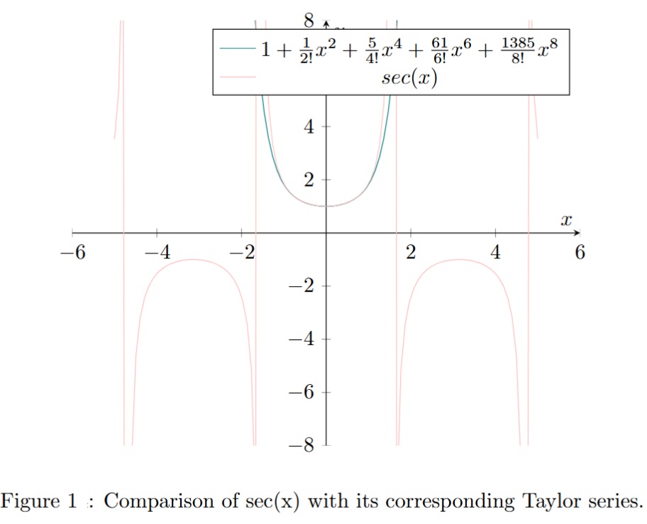
In the previous post we have computed the Padé approximants for the $exp(x)$ function. The approximation was not very impressive compared to the Maclaurin series of $exp()$ since the latter converges for all $x$ . In this post we will have a look at the Padé approximants and Maclaurin series of $sec(x)$ .

First let’s recall the graph of $sec(x)$ (see figure 1). $sec(x)$ is a function with vertical asymptotes that cannot be approximated globally by a Taylor series. The Maclaurin series of $sec(x)$ is:

$\displaystyle sec(x) = 1 + \frac{1}{2!}x^2 + \frac{5}{4!} x^4 + \frac{61}{6!} x^6 + \frac{1385}{8!} x^8 + \cdots$

$\displaystyle = \sum_{n=0}^{\infty} \frac{E_n}{(2n)!} x^{2n}$

Where $E_n$ are so-called Euler numbers:

$\displaystyle E_1 = 1, \quad E_2 = 5, \quad E_3 = 61, \quad E_4 = 1385, \quad E_5 = 50521, \quad E_6 = 2702765$

We would like to compute the $P(4,4)$ approximant of $sec(x)$ . The first step is to have a look at the corresponding Hankel determinant (which is the determinant of the Hankel matrix):

$\displaystyle H_{n,m}(f) = \det \left( \begin{array}{cccc} C_{m-n+1} & C_{m-n+2} & \cdots & C_m \\ C_{m-n+2} & C_{m-n+3} & \cdots & C_{m+1} \\ \vdots & \vdots & \ddots & \vdots \\ C_m & C_{m+1} & \cdots & C_{m+n-1} \end{array} \right)$

For $m = 4$ and $n = 4$ we have:

$\displaystyle H_{4,4}(f) = \det \left( \begin{array}{cccc} C_1 & C_2 & C_3 & C_4 \\ C_2 & C_3 & C_4 & C_5 \\ C_3 & C_4 & C_5 & C_6 \\ C_4 & C_5 & C_6 & C_7 \end{array} \right)$

and the corresponding Hankel determinant for the $P(4,4)$ of $sec(x)$ is:

$\displaystyle H_{4,4}(sec(x)) = \det \left( \begin{array}{cccc} 0 & \frac{1}{2!} & 0 & \frac{5}{4!} \\ \frac{1}{2!} & 0 & \frac{5}{4!} & 0 \\ 0 & \frac{5}{4!} & 0 & \frac{61}{6!} \\ \frac{5}{4!} & 0 & \frac{61}{6!} & 0 \end{array} \right) = 1.08507 \times 10^{-6}$

the determinant being not equal to zero implies that we can inverse the Hankel matrix and solve the systems to compute the Padé coefficients of $P(4,4)$ for $sec(x)$ (see post Computing Padé approximants). The inverse of the Hankel matrix is given by:

$\displaystyle \left( \begin{array}{cccc} 0 & -81.3333 & 0 & 200 \\ -81.3333 & 0 & 200 & 0 \\ 0 & 200 & 0 & -480 \\ 200 & 0 & -480 & 0 \end{array} \right)$

We have to solve this first linear system:

$\displaystyle \left( \begin{array}{cccc} 0 & \frac{1}{2!} & 0 & \frac{5}{4!} \\ \frac{1}{2!} & 0 & \frac{5}{4!} & 0 \\ 0 & \frac{5}{4!} & 0 & \frac{61}{6!} \\ \frac{5}{4!} & 0 & \frac{61}{6!} & 0 \end{array} \right) \left( \begin{array}{c} B_4 \\ B_3 \\ B_2 \\ B_1 \end{array} \right) = - \left( \begin{array}{c} C_5 \\ C_6 \\ C_7 \\ C_8 \end{array} \right) = \left( \begin{array}{c} 0 \\ -\frac{61}{6!} \\ 0 \\ -\frac{1385}{8!} \end{array} \right)$

$\displaystyle \left( \begin{array}{cccc} 0 & \frac{1}{2!} & 0 & \frac{5}{4!} \\ \frac{1}{2!} & 0 & \frac{5}{4!} & 0 \\ 0 & \frac{5}{4!} & 0 & \frac{61}{6!} \\ \frac{5}{4!} & 0 & \frac{61}{6!} & 0 \end{array} \right)^{-1} \left( \begin{array}{c} 0 \\ -\frac{61}{6!} \\ 0 \\ -\frac{1385}{8!} \end{array} \right) = \left( \begin{array}{c} B_4 \\ B_3 \\ B_2 \\ B_1 \end{array} \right)$

$\displaystyle \left( \begin{array}{cccc} 0 & -81.3333 & 0 & 200 \\ -81.3333 & 0 & 200 & 0 \\ 0 & 200 & 0 & -480 \\ 200 & 0 & -480 & 0 \end{array} \right) \left( \begin{array}{c} 0 \\ -\frac{61}{6!} \\ 0 \\ -\frac{1385}{8!} \end{array} \right) = \left( \begin{array}{c} \frac{104.3191}{5040} \\ 0 \\ -\frac{115}{252} \\ 0 \end{array} \right)$

Solving the system above allows us to compute the $B_n$ coefficients (see results below). Now, according to the calculations presented in the post (see Computing Padé approximants), we have to solve the second linear system to compute the $A_m$ coefficients:

$\displaystyle \left( \begin{array}{ccccc} C_0 & 0 & 0 & 0 & 0 \\ C_1 & C_0 & 0 & 0 & 0 \\ C_2 & C_1 & C_0 & 0 & 0 \\ C_3 & C_2 & C_1 & C_0 & 0 \\ C_4 & C_3 & C_2 & C_1 & C_0 \end{array} \right) \left( \begin{array}{c} 1 \\ B_1 \\ B_2 \\ B_3 \\ B_4 \end{array} \right) = \left( \begin{array}{c} A_0 \\ A_1 \\ A_2 \\ A_3 \\ A_4 \end{array} \right)$

$\displaystyle \left( \begin{array}{ccccc} 1 & 0 & 0 & 0 & 0 \\ 0 & 1 & 0 & 0 & 0 \\ \frac{1}{2!} & 0 & 1 & 0 & 0 \\ 0 & \frac{1}{2!} & 0 & 1 & 0 \\ \frac{5}{4!} & 0 & \frac{1}{2!} & 0 & 1 \end{array} \right) \left( \begin{array}{c} 1 \\ 0 \\ -\frac{115}{252} \\ 0 \\ \frac{104.3191}{5040} \end{array} \right) = \left( \begin{array}{c} A_0 \\ A_1 \\ A_2 \\ A_3 \\ A_4 \end{array} \right)$

$\displaystyle A_0 = 1, \quad A_1 = 0, \quad A_2 = \frac{1}{2!} - \frac{115}{252} = \frac{11}{252}, \quad A_3 = 0, \quad A_4 = \frac{5}{24} - \frac{115}{504} + \frac{104.3191}{5040} = \frac{4.3191}{5040}$

$\displaystyle B_0 = 1, \quad B_1 = 0, \quad B_2 = -\frac{115}{252}, \quad B_3 = 0, \quad B_4 = \frac{104.3191}{5040}$

This implies that for $sec(x)$ :

$\displaystyle P(4,4) = \frac{1 + A_2 x^2 + A_4 x^4}{1 + B_2 x^2 + B_4 x^4}$

$\displaystyle = \frac{1 + \frac{11}{252} x^2 + \frac{4.3191}{5040} x^4}{1 - \frac{115}{252} x^2 + \frac{104.3191}{5040} x^4}$

The graph of $P(4,4)$ for $sec(x)$ is presented in figure 2. The graph of $sec(x)$ and its corresponding $P(4,4)$ is presented in figure 3. We can see that the $P(4,4)$ approximant (in green) is approximating the function $sec(x)$ beyond its vertical asymptotes (pink vertical lines) in contrast to the corresponding Taylor series presented in figure 1. Moreover the convergence of $P(4,4)$ is better than the one of the Taylor series.

It is also interesting to note that the ‘information’ needed to construct the Padé approximants of the function $sec(x)$ has been extracted from the truncated Taylor series. Despite this fact, the Padé approximant provides a better approximation of the $sec(x)$ function than the series from which it is derived.

July 24, 2025

Padé approximants of exp(x)

We can organize and present the Padé $P(m,n)$ approximants in a table like this:

$P(m,n)$	0	1	2	3	$...$
0	$P(0,0)$	$P(1,0)$	$P(2,0)$	$P(3,0)$	$...$
1	$P(0,1)$	$P(1,1)$	$P(2,1)$	$P(3,1)$	$...$
2	$P(0,2)$	$P(1,2)$	$P(2,2)$	$P(3,2)$	$...$
3	$P(0,3)$	$P(1,3)$	$P(2,3)$	$P(3,3)$	$...$
$...$	$...$	$...$	$...$	$...$	$...$

The table above shows, in order, Padé’s first approximants. This is a way to present and organize the Padé approximants. We can use the procedure presented in the previous posts to compute the Padé approximants for the exponential function $\exp(x)$ . Solving systems presented in the previous posts, leads to the following table:

$P(m,n)$	0	1	2	3	$...$
0	$1$	$1 + x$	$1 + x + \frac{x^2}{2}$	$1 + x + \frac{x^2}{2} + \frac{x^3}{6}$	$...$
1	$\frac{1}{1 - x}$	$\frac{1 + \frac{1}{2}x}{1 - \frac{1}{2}x}$	$\frac{1 + \frac{2}{3}x + \frac{1}{6}x^2}{1 - \frac{1}{3}x}$	$\frac{1 + \frac{3}{4}x + \frac{1}{4}x^2 + \frac{1}{24}x^3}{1 - \frac{1}{4}x}$	$...$
2	$\frac{1}{1 - x + \frac{1}{2}x^2}$	$\frac{1 + \frac{1}{3}x}{1 - \frac{2}{3}x + \frac{1}{6}x^2}$	$\frac{1 + \frac{1}{2}x + \frac{1}{12}x^2}{1 - \frac{1}{2}x + \frac{1}{12}x^2}$	$\frac{1 + \frac{3}{5}x + \frac{3}{20}x^2 + \frac{1}{60}x^3}{1 - \frac{2}{5}x + \frac{1}{20}x^2}$	$...$
3	$\frac{1}{1 - x + \frac{1}{2}x^2 - \frac{1}{6}x^3}$	$\frac{1 + \frac{1}{4}x}{1 - \frac{3}{4}x + \frac{1}{4}x^2 - \frac{1}{24}x^3}$	$\frac{1 + \frac{2}{5}x + \frac{1}{20}x^2}{1 - \frac{3}{5}x + \frac{3}{20}x^2 - \frac{1}{60}x^3}$	$\frac{1 + \frac{1}{2}x + \frac{1}{10}x^2 + \frac{1}{120}x^3}{1 - \frac{1}{2}x + \frac{1}{10}x^2 - \frac{1}{120}x^3}$	$...$
$...$	$...$	$...$	$...$	$...$	$...$

Setting x = 1, we obtain the following values:

$P(m,n)$	0	1	2	3
0	$1.000000$	$2.000000$	$2.500000$	$2.666667$
1	—	$3.000000$	$2.750000$	$2.722222$
2	$2.000000$	$2.666667$	$2.714286$	$2.717949$
3	$3.000000$	$2.727273$	$2.718750$	$2.718310$

The ‘relative error’ is defined as:

$\displaystyle \text{Relative error} := \frac{\text{Approximation} - \text{Exact value}}{\text{Exact value}}$

Relative errors of Padé approximants $P(m,n)$ of $e^x$ evaluated at x = 1, using the exact value $e \approx 2.718281$ are shown in the table below:

$P(m,n)$	0	1	2	3
0	$-0.632121$	$-0.264241$	$-0.080301$	$-0.018988$
1	—	$0.103638$	$0.011662$	$0.001449$
2	$-0.264241$	$-0.018988$	$-0.001471$	$-0.000122$
3	$0.103638$	$0.003307$	$0.000172$	$0.000010$

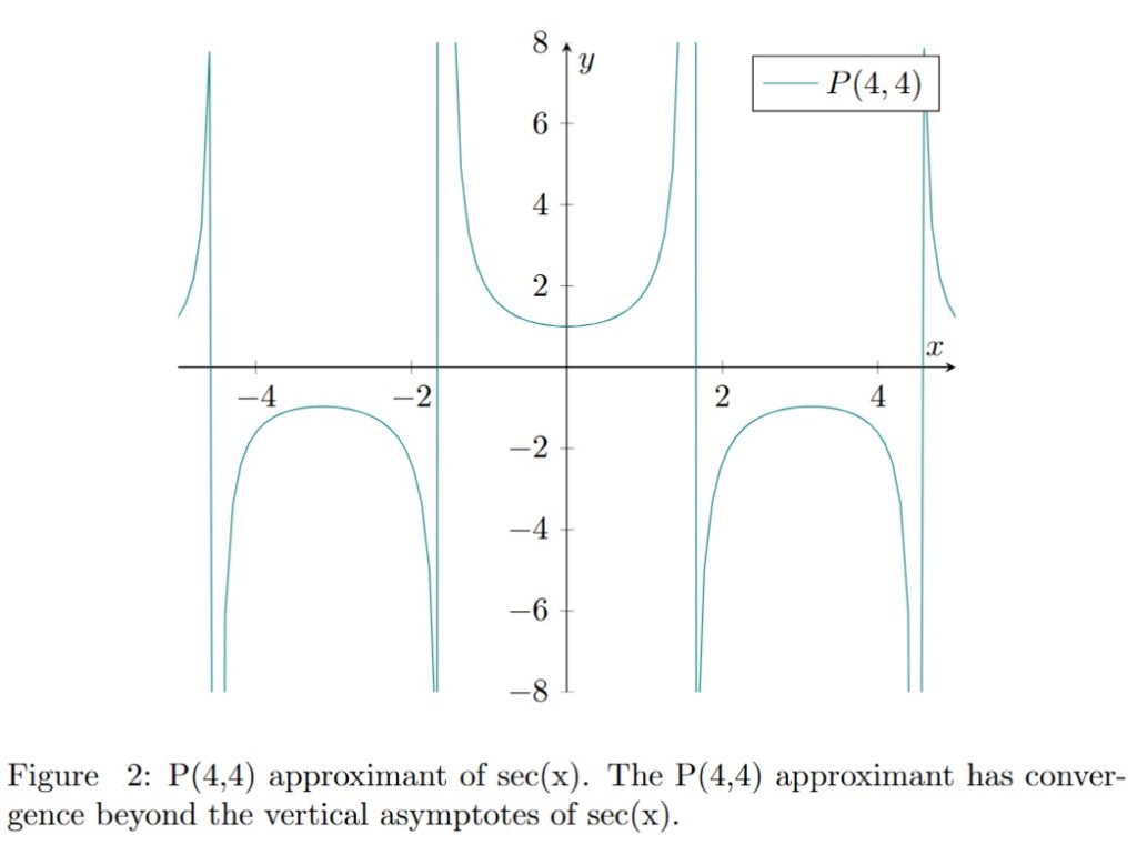
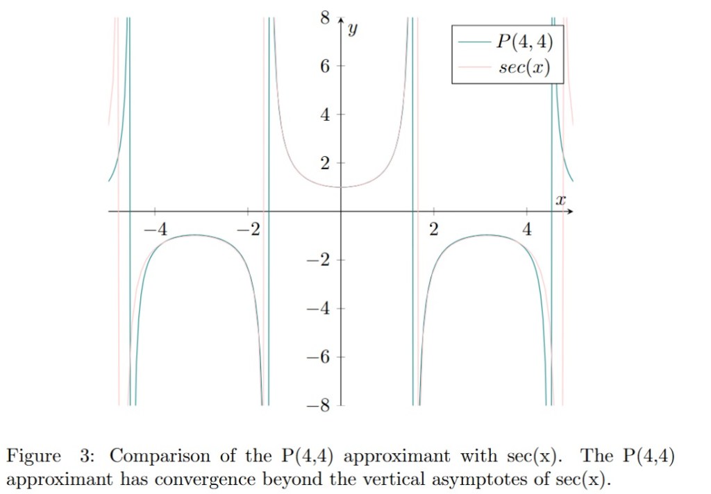
The Padé approximants exhibit an alternating sign pattern in their relative errors. This indicates that the Padé approximants oscillate around the true value $e$ , approaching it from both sides. In contrast, the Taylor approximations converge monotonically from below.

July 17, 2025

Hankel determinant

In the previous posts, we have seen that in order to compute the Padé coefficients $P(m,n)$ corresponding to a given geometric series we have to be invert the following matrix:

$\displaystyle \begin{pmatrix} C_{m-n+1} & C_{m-n+2} & \ldots & C_{m} \\ C_{m-n+2} & C_{m-n+3} & \ldots & C_{m+1} \\ \vdots & & & \vdots \\ C_{m} & C_{m+1} & \ldots & C_{m+n-1} \end{pmatrix}$

Where $C_l$ are the coefficients of the Taylor series. The matrix above is called a “Hankel matrix”. A ‘Hankel Matrix’ is a symmetric square matrix in which each ascending skew-diagonal from left to right is constant. For Example a Hankel matrix of size 5 can be written like this:

$\displaystyle \begin{pmatrix} a & b & c & d & e \\ b & c & d & e & f \\ c & d & e & f & g \\ d & e & f & g & h \\ e & f & g & h & i \end{pmatrix}$

Let’s make some observations on the Hankel determinant $H_{n,m}(f)$ :

$\displaystyle H_{n,m}(f) := \begin{vmatrix} C_{m-n+1} & C_{m-n+2} & \ldots & C_{m} \\ C_{m-n+2} & C_{m-n+3} & \ldots & C_{m+1} \\ \vdots & & & \vdots \\ C_{m} & C_{m+1} & \ldots & C_{m+n-1} \end{vmatrix}$

This determinant has n colons and n rows. We can also numerate the terms of the determinant following the notation:

$\displaystyle H_{n,m}(f) := \begin{vmatrix} d(1,1) & d(1,2) & \ldots & d(1,n) \\ d(2,1) & d(2,2) & \ldots & d(2,n) \\ \vdots & & & \vdots \\ d(n,1) & d(n,2) & \ldots & d(n,n) \end{vmatrix}$

Where $d(1,1) := C_{m-n+1}$ etc. This notation of the terms of the determinants implies that:

$\displaystyle d(i,j) = C_{m-n+i+j-1}$

So that:

$\displaystyle d(1,1) = C_{m-n+1+1-1} = C_{m-n+1}$

$\displaystyle d(1,2) = C_{m-n+1+2-1} = C_{m-n+2}$

$\displaystyle d(2,1) = C_{m-n+2+1-1} = C_{m-n+2}$

$\displaystyle \ldots$

$\displaystyle d(n,n) = C_{m-n+n+n-1} = C_{m+n-1}$

If $f(x)$ is a even function of class $C_{\infty}$ , we see that odd coefficients $C_{2p+1} = \frac{f^{(2p+1)}(0)}{(2p+1)!} = 0$ . In this case, every second term of in the Hankel matrix is zero. If $f(x)$ is even, we can establish that if $m$ and $n$ are odd then the Hankel determinant is zero:

The term with index $d(i,j)$ of the Hankel determinant is $C_{m-n+i+j-1}$ . As stated before, this term is zero for an even function if $m-n+i+j-1$ is odd. Now, if $m$ and $n$ are odd this means that $n-m$ is even and $m-n+i+j-1$ is odd when $i + j$ is even. It follows that, in the case of an even function, the Hankel determinant is of the form:

$\displaystyle \begin{vmatrix} 0 & b & 0 & d & \hdots \\ b & 0 & d & 0 & \hdots \\ 0 & d & 0 & f & \hdots \\ \vdots & \vdots & \vdots & & \ddots \end{vmatrix}$

We observe that the odd rows of this determinant are linear combinations of:

$\displaystyle \begin{pmatrix} 0 \\ 1 \\ 0 \\ 0 \\ 0 \\ \vdots \end{pmatrix}, \begin{pmatrix} 0 \\ 0 \\ 0 \\ 1 \\ 0 \\ \vdots \end{pmatrix} \text{, etc.}$

This implies that odd-numbered columns are linked and therefore the determinant is zero.

As example we will derive the $P(3,3)$ of the cosine function. First we have to consider the geometric series of degrees up to $3 + 3 = 6$ of cosine:

$\displaystyle \cos x = 1 - \frac{x^2}{2!} + \frac{x^4}{4!} - \frac{x^6}{6!} + \mathcal{O}(x^8)$

For $m=3$ and $n=3$ ( $m$ and $n$ are both odd) the Hankel determinant is:

$\displaystyle H_{3,3}(f) = \begin{vmatrix} C_{1} & C_{2} & C_{3} \\ C_{2} & C_{3} & C_{4} \\ C_{3} & C_{4} & C_{5} \end{vmatrix}$

The corresponding Hankel determinant for calculating the coefficients of the $P(3,3)$ Padé approximant of the geometric series of cosine is therefore:

$\displaystyle H_{3,3}(cos) = \begin{vmatrix} 0 & -\frac{1}{2} & 0 \\ -\frac{1}{2} & 0 & \frac{1}{4!} \\ 0 & \frac{1}{4!} & 0 \end{vmatrix} = 0$

This implies that we cannot calculate the $P(3,3)$ approximant for the cosine function.

In conclusion, for an even function like cosine, when m and n are odd, the Hankel determinant H_n,m(f) is zero due to the linear dependence of the columns.

July 10, 2025
Padé approximants of sin(x)

We are interested in the $P(2,2)$ Padé approximant of the sinus function. We first have to consider de Taylor series of $sin(x)$ up to terms $2+2=4$ :

$\displaystyle sin(x) = x - \frac{x^3}{3!} + \mathcal{O}(x^5)$

For $m=2$ and $n=2$ , the Hankel determinant (see previous post) is:

$\displaystyle H_{2,2}(f) = \begin{vmatrix} C_{1} & C_{2} \\ C_{2} & C_{3} \\ \end{vmatrix}$

The Hankel determinant corresponding to the sinus series above is therefore:

$\displaystyle H_{2,2}(sin) = \begin{vmatrix} 1 & 0 \\ 0 & -\frac{1}{6} \\ \end{vmatrix} = -\frac{1}{6}$

According to the previous section we have to first solve:

$\displaystyle \begin{pmatrix} 1 & 0 \\ 0 & -\frac{1}{6} \end{pmatrix} \begin{pmatrix} B_2 \\ B_1 \end{pmatrix} = - \begin{pmatrix} C_{3} \\ C_{4} \\ \end{pmatrix}$

Since $C_3 = -\frac{1}{6}$ and $C_4 = 0$ we have to solve:

$\displaystyle \begin{pmatrix} 1 & 0 \\ 0 & -\frac{1}{6} \end{pmatrix} \begin{pmatrix} B_2 \\ B_1 \end{pmatrix} = \begin{pmatrix} \frac{1}{6} \\ 0 \\ \end{pmatrix}$

So $B_2 = \frac{1}{6}$ and $B_1 = 0$ .

Finally we have to solve this system ( $B_0$ being set to one):

$\displaystyle \begin{pmatrix} C_0 & 0 & 0 \\ C_1 & C_0 & 0 \\ C_2 & C_1 & C_0 \end{pmatrix} \begin{pmatrix} 1 \\ B_1 \\ B_2 \end{pmatrix} = \begin{pmatrix} A_0 \\ A_1 \\ A_2 \end{pmatrix}$

$\displaystyle \begin{pmatrix} 0 & 0 & 0 \\ 1 & 0 & 0 \\ 0 & 1 & 0 \end{pmatrix} \begin{pmatrix} 1 \\ 0 \\ \frac{1}{6} \end{pmatrix} = \begin{pmatrix} A_0 \\ A_1 \\ A_2 \end{pmatrix}$

This implies that $A_0 = 0$ , $A_1 = 1$ and $A_2 = 0$ . The $P(2,2)$ Padé approximant for $sin(x)$ is therefore:

$\displaystyle P(2,2) = \frac{x}{1 + \frac{1}{6}x^2}$

The graph of $sin(x)$ and its corresponding $P(2,2)$ approximant are shown in figure 1.

July 3, 2025