Month: June 2025

Computing Padé approximants

We have seen that Padé approximants offer a more efficient and flexible method for approximating functions than the Taylor expansion. They have been used in many areas of mathematics and physics.

We would like to find a more convenient way to calculate the Padé coefficients of any Taylor or Maclaurin series.

In the following post, we admit the existence of Padé approximants $P(m,n)$ . It is generally possible to find the coefficients of the Padé approximants except in the case of degeneracy due to particular values of the coefficients of the corresponding series. We will not consider these cases in the rest of our study. Remember that we defined Padé approximants as rational functions:

$\displaystyle P(m,n) := \frac{A_0 + A_1 x + A_2 x^2 + \dots + A_m x^m}{1 + B_1 x + B_2 x^2 + \dots + B_n x^n}$

If we want to solve a very hard or even impossible-to-solve-exactly problem using perturbation theory we will end up with a power series like $\sum_{k=0}^{l} C_k x^k$ . To convert this (potentially not converging) series to its corresponding Padé approximant we write (as described in the previous post):

$\displaystyle \frac{A_0 + A_1 x + \dots + A_m x^m}{1 + B_1 x + \dots + B_n x^n} = C_0 + C_1 x + \dots + C_{n+m}x^{n+m} + \mathcal{O}(x^{m+n+1})$

From a purely algorithmic point of view and in order to calculate the Padé coefficients we drop $\mathcal{O}(x^{m+n+1})$ :

$\displaystyle (C_0 + C_1 x + \dots + C_{n+m}x^{n+m})(1 + B_1 x + \dots + B_n x^n) - (A_0 + A_1 x + \dots + A_m x^m) = 0$

$\displaystyle \sum_{i=0}^{n+m}\sum_{j=0}^{n}C_iB_jx^{i+j} - (A_0 + A_1 x + \dots + A_m x^m)= 0$

Comparing each term of the geometric series on the right and the left of this equation (Uniqueness of power series coeffficients) we obtain the following set of equations:

$\displaystyle (C_0 B_0 - A_0) = 0 \quad (i+j = 0)$
$\displaystyle (C_1 B_0 + C_0 B_1 - A_1)x = 0 \quad (i+j = 1)$
$\displaystyle (C_2 B_0 + C_1 B_1 + C_0 B_2 - A_2)x^2 = 0 \quad (i+j = 2)$
$\dots$
$\displaystyle (C_m B_0 + C_{m-1} B_1 + \dots + C_{m-n} B_n - A_m)x^m = 0 \quad (i+j = m)$
$\displaystyle (C_{m+1} B_0 + C_m B_1 + \dots + C_{m-n+1} B_n)x^{m+1} = 0 \quad (i+j = m+1)$
$\dots$
$\displaystyle (C_{m+n} B_0 + C_{m+n-1} B_1 + \dots + C_m B_n)x^{m+n} = 0 \quad (i+j = m+n)$

Using $A_k = 0$ for $k > m$ . We can split this system of equations in two parts and get rid of the x-terms. One part containing the $A_i$ coefficients (up to i+j = m) and the part without $A_i$ coefficients. The first system of equation is:

$\displaystyle C_0 B_0 - A_0 = 0$
$\displaystyle C_1 B_0 + C_0 B_1 - A_1 = 0$
$\displaystyle C_2 B_0 + C_1 B_1 + C_0 B_2 - A_2 = 0$
$\dots$
$\displaystyle C_m B_0 + C_{m-1} B_1 + \dots + C_{m-n} B_n - A_m = 0$

The second system of equations:

$\displaystyle C_{m+1} B_0 + C_m B_1 + \dots + C_{m-n+1} B_n = 0$
$\dots$
$\displaystyle C_{m+n} B_0 + C_{m+n-1} B_1 + \dots + C_m B_n = 0$

Setting $B_0 = 1$ without loss of generality the second system of equations becomes:

$\displaystyle C_m B_1 + \dots + C_{m-n+1} B_n = -C_{m+1}$
$\displaystyle C_{m+1} B_1 + \dots + C_{m-n+2} B_n = -C_{m+2}$
$\dots$
$\displaystyle C_{m+n-1} B_1 + \dots + C_m B_n = -C_{m+n}$

Changing the order of the coefficients gives:

$\displaystyle C_{m-n+1} B_n + \dots + C_m B_1 = -C_{m+1}$
$\displaystyle C_{m-n+2} B_n + \dots + C_{m+1} B_1 = -C_{m+2}$
$\dots$
$\displaystyle C_m B_n + \dots + C_{m+n-1} B_1 = -C_{m+n}$

We can write both systems using matrix notation:

$\displaystyle \left( \begin{array}{cccccc} C_0 & 0 & \dots & & & 0 \\ C_1 & C_0 & 0 & \dots & & 0 \\ C_2 & C_1 & C_0 & 0 & \dots & 0 \\ \vdots & & & & & \vdots \\ C_m & \dots & & & \dots & C_{m-n} \end{array} \right) \left( \begin{array}{c} B_0 \\ B_1 \\ B_2 \\ \vdots \\ B_n \end{array} \right) = \left( \begin{array}{c} A_0 \\ A_1 \\ A_2 \\ \vdots \\ A_m \end{array} \right)$
$\displaystyle \left( \begin{array}{ccccc} C_{m-n+1} & C_{m-n+2} & \dots & & C_m \\ C_{m-n+2} & C_{m-n+3} & \dots & & C_{m+1} \\ \vdots & & & & \vdots \\ C_m & C_{m+1} & & \dots & C_{m+n-1} \end{array} \right) \left( \begin{array}{c} B_n \\ B_{n-1} \\ \vdots \\ B_1 \end{array} \right) = - \left( \begin{array}{c} C_{m+1} \\ C_{m+2} \\ \vdots \\ C_{m+n} \end{array} \right)$

Practically, we start calculations where $m-n+k \geq 0$ . The resolution of the second system gives the values of the $B_j$ coefficients which are injected into the first system to obtain the $A_i$ coefficient (using $B_0 = 1$ ). So if the following determinant (called a ‘Hankel determinant’):

$\displaystyle H_{n,m}(f) := \left| \begin{array}{ccccc} C_{m-n+1} & C_{m-n+2} & \dots & & C_m \\ C_{m-n+2} & C_{m-n+3} & \dots & & C_{m+1} \\ \vdots & & & & \vdots \\ C_m & C_{m+1} & & \dots & C_{m+n-1} \end{array} \right|$

Is not null. i.e.:

$\displaystyle H_{n,m}(f) \neq 0$

the Padé approximant will be unique. The calculations for the Padé approximant coefficients yield a unique solution for any Taylor or Maclaurin series, provided the Hankel determinant is not null, excluding cases of degeneracy due to specific coefficient values.

June 26, 2025
Padé approximants

We would like to represent functions using continued fractions (similarly as we did for numbers). For example, a well-known continued fraction representing $tan(x)$ is:

$\displaystyle tan(x) = \frac{x}{1 - \frac{x^2}{3 - \frac{x^2}{5 - \frac{x^2}{7 - \cdots}}}}$

Continued fractions like this one typically have a bigger definition domain compared to the corresponding Taylor series. This is illustrated graphically in figure 1 and figure 2.

The continued fraction representation of a function seems a promising approach since the radius of convergence ‘seems’ at a first glance much bigger and the approximation ‘looks’ much better (i.e. converging faster) than for Taylor and Maclaurin series. We will illustrate these statements.

In order to make some progress in the construction of continued fractions corresponding to functions, we’ll start by defining the following rational functions, which will prove to have interesting properties in their own right:

$\displaystyle P(1,1) := \frac{A_0 + A_1 x}{1 + B_1 x}$

$\displaystyle P(2,1) := \frac{A_0 + A_1 x + A_2 x^2}{1 + B_1 x}$

$\displaystyle P(2,2) := \frac{A_0 + A_1 x + A_2 x^2}{1 + B_1 x + B_2 x^2}$

$\displaystyle \cdots$

$\displaystyle P(m,n) := \frac{A_0 + A_1 x + A_2 x^2 + \cdots + A_m x^m}{1 + B_1 x + B_2 x^2 + \cdots + B_n x^n}$

Using the definitions above we present some examples using the first terms of the Maclaurin series of $tan(x)$ :

$\displaystyle \frac{A_0 + A_1 x + A_2 x^2}{1 + B_1 x + B_2 x^2} = x + \frac{1}{3} x^3$

$\displaystyle A_0 + A_1 x + A_2 x^2 = (x + \frac{1}{3} x^3) (1 + B_1 x + B_2 x^2)$

$\displaystyle A_0 + A_1 x + A_2 x^2 = x + B_1 x^2 + B_2 x^3 + \frac{1}{3} x^3 + \frac{1}{3} B_1 x^4 + \frac{1}{3} B_2 x^5$

$\displaystyle A_0 + A_1 x + A_2 x^2 = x + B_1 x^2 + \left(B_2 + \frac{1}{3}\right) x^3 + \frac{1}{3} B_1 x^4 + \frac{1}{3} B_2 x^5$

In the example above we are considering a $P(2,2)$ rational function. So we consider up to 2 + 2 = 4 as the maximum degree we would like to consider for further computations. The equation above becomes:

$\displaystyle A_0 + A_1 x + A_2 x^2 = x + B_1 x^2 + \left(B_2 + \frac{1}{3}\right) x^3 + \frac{1}{3} B_1 x^4$

Comparing the coefficients of both sides we obtain:

$\displaystyle A_0 = 0 \quad \text{and} \quad B_2 + \frac{1}{3} = 0$

$\displaystyle A_1 = 1 \quad \text{and} \quad \frac{1}{3} B_1 = 0$

$\displaystyle A_2 = B_1$

Solving the set of equations above gives:

$\displaystyle A_0 = 0, \ A_1 = 1, \ A_2 = 0, \ B_1 = 0, \ B_2 = -\frac{1}{3}$

$\displaystyle \implies P(2,2) := \frac{A_0 + A_1 x + A_2 x^2}{1 + B_1 x + B_2 x^2} = \frac{x}{1 - \frac{1}{3} x^2}$

This is clearly the first term of the continued fraction of $tan(x)$ as shown above.

$P(m,n)$ as defined above are called Padé approximants. A Padé approximant is the “best” approximation of a function near a specific point by a rational function of given order. We also have convergence beyond the radius of convergence of the corresponding series.

Let’s calculate the $P(1,2)$ corresponding to the first terms of the Maclaurin series of $tan(x)$ . 1 + 2 = 3 implies that we have to consider the Taylor series up to degree 3.

$\displaystyle \frac{A_0 + A_1 x}{1 + B_1 x + B_2 x^2} = x + \frac{1}{3} x^3$

$\displaystyle A_0 + A_1 x = (x + \frac{1}{3} x^3) (1 + B_1 x + B_2 x^2)$

$\displaystyle A_0 + A_1 x = x + B_1 x^2 + B_2 x^3 + \frac{1}{3} x^3 + \frac{1}{3} B_1 x^4 + \frac{1}{3} B_2 x^5$

$\displaystyle A_0 + A_1 x = x + B_1 x^2 + \left(B_2 + \frac{1}{3}\right) x^3 + \frac{1}{3} B_1 x^4 + \frac{1}{3} B_2 x^5$

Keeping only degrees up to 3:

$\displaystyle A_0 + A_1 x = x + B_1 x^2 + \left(B_2 + \frac{1}{3}\right) x^3$

Comparing the coefficients of both sides we obtain:

$\displaystyle A_0 = 0 \quad \text{and} \quad B_1 = 0$

$\displaystyle A_1 = 1 \quad \text{and} \quad B_2 + \frac{1}{3} = 0 \implies B_2 = -\frac{1}{3}$

$\displaystyle \implies P(1,2) := \frac{A_0 + A_1 x}{1 + B_1 x + B_2 x^2} = \frac{x}{1 - \frac{1}{3} x^2}$

We observe that (in this case):

$\displaystyle P(1,2) = P(2,2)$

Now we calculate the $P(3,3)$ corresponding to the first terms of the Maclaurin series of $tan(x)$ . 3 + 3 = 6 implies that we have to consider the Taylor series up to degree 5:

$\displaystyle \frac{A_0 + A_1 x + A_2 x^2 + A_3 x^3}{1 + B_1 x + B_2 x^2 + B_3 x^3} = x + \frac{1}{3} x^3 + \frac{2}{15} x^5$

$\displaystyle A_0 + A_1 x + A_2 x^2 + A_3 x^3 = (x + \frac{1}{3} x^3 + \frac{2}{15} x^5) (1 + B_1 x + B_2 x^2 + B_3 x^3)$

$\displaystyle A_0 + A_1 x + A_2 x^2 + A_3 x^3 = x + B_1 x^2 + B_2 x^3 + B_3 x^4 + \frac{1}{3} x^3 + \frac{1}{3} B_1 x^4 + \frac{1}{3} B_2 x^5 + \frac{1}{3} B_3 x^6 + \frac{2}{15} x^5 + \frac{2}{15} B_1 x^6 + \frac{2}{15} B_2 x^7 + \frac{2}{15} B_3 x^8$

$\displaystyle A_0 + A_1 x + A_2 x^2 + A_3 x^3 = x + B_1 x^2 + \left(B_2 + \frac{1}{3}\right) x^3 + \left(B_3 + \frac{1}{3} B_1\right) x^4 + \left(\frac{1}{3} B_2 + \frac{2}{15}\right) x^5 + \left(\frac{1}{3} B_3 + \frac{2}{15} B_1\right) x^6 + \frac{2}{15} B_2 x^7 + \frac{2}{15} B_3 x^8$

Keeping only degrees up to 6:

$\displaystyle A_0 + A_1 x + A_2 x^2 + A_3 x^3 = x + B_1 x^2 + \left(B_2 + \frac{1}{3}\right) x^3 + \left(B_3 + \frac{1}{3} B_1\right) x^4 + \left(\frac{1}{3} B_2 + \frac{2}{15}\right) x^5 + \left(\frac{1}{3} B_3 + \frac{2}{15} B_1\right) x^6$

This implies:

$\displaystyle A_0 = 0 \quad \text{and} \quad B_3 + \frac{1}{3} B_1 = 0$

$\displaystyle A_1 = 1 \quad \text{and} \quad \frac{1}{3} B_2 + \frac{2}{15} = 0$

$\displaystyle A_2 = B_1 \quad \text{and} \quad \frac{1}{3} B_3 + \frac{2}{15} B_1 = 0$

$\displaystyle A_3 = B_2 + \frac{1}{3}$

Solving the set of equations above gives:

$\displaystyle A_0 = 0, \ A_1 = 1, \ A_2 = 0, \ A_3 = -\frac{1}{15}, \ B_1 = 0, \ B_2 = -\frac{2}{5}, \ B_3 = 0$

$\displaystyle \implies P(3,3) := \frac{A_0 + A_1 x + A_2 x^2 + A_3 x^3}{1 + B_1 x + B_2 x^2 + B_3 x^3} = \frac{x - \frac{1}{15} x^3}{1 - \frac{6}{15} x^2}$

Now consider the first terms of the continued fraction of $tan(x)$ :

$\displaystyle \frac{x}{1 - \frac{x^2}{3 - \frac{x^2}{5}}} = \frac{x}{1 - \frac{x^2}{\frac{15 - x^2}{5}}} = \frac{x}{1 - \frac{5 x^2}{15 - x^2}} = \frac{15 x - x^3}{15 - x^2 - 5 x^2} = \frac{15 x - x^3}{15 - 6 x^2}$

$\displaystyle \implies P(3,3) = \frac{x - \frac{1}{15} x^3}{1 - \frac{6}{15} x^2} = \frac{x}{1 - \frac{x^2}{3 - \frac{x^2}{5}}}$

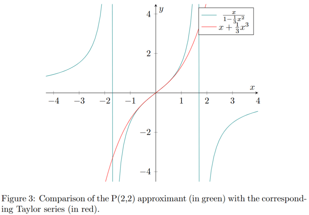
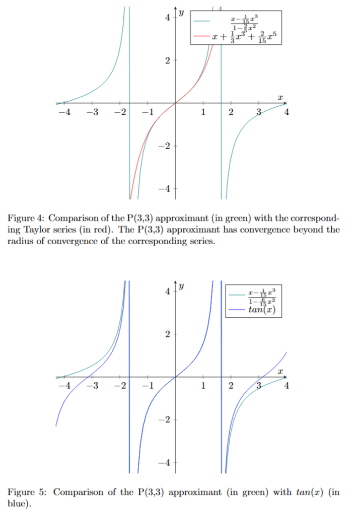
Therefore, the $P(1,1)$ , $P(2,2)$ and $P(3,3)$ Padé approximants (see fig. 3, 4 and 5) of $tan(x)$ are equivalent to the first terms of its continued fraction as presented above.

The results above about $tan(x)$ suggest that a “Padé transformation” (i.e. converting a series into a rational function using the procedure described above) of a divergent Maclaurin and Taylor series is converging beyond the radius of convergence of the Maclaurin series.

This gives hope for the use of divergent series as often encountered in perturbation theory.

We would like to calculate the $P(m,n)$ of $exp(x)$ . First, we would like to calculate $P(1,1)$ . We, therefore, consider the Maclaurin series of $exp(x)$ up to 1 + 1 = 2 degrees:

$\displaystyle \frac{A_0 + A_1 x}{1 + B_1 x} = 1 + x + \frac{1}{2} x^2$

$\displaystyle A_0 + A_1 x = (1 + x + \frac{1}{2} x^2)(1 + B_1 x)$

$\displaystyle A_0 + A_1 x = 1 + B_1 x + x + B_1 x^2 + \frac{1}{2} x^2 + \frac{1}{2} B_1 x^3$

$\displaystyle A_0 + A_1 x = 1 + (B_1 + 1) x + \left(B_1 + \frac{1}{2}\right) x^2 + \frac{1}{2} B_1 x^3$

Keeping only degrees up to 2:

$\displaystyle A_0 + A_1 x = 1 + (B_1 + 1) x + \left(B_1 + \frac{1}{2}\right) x^2$

This implies:

$\displaystyle A_0 = 1 \quad \text{and} \quad B_1 + \frac{1}{2} = 0$

$\displaystyle A_1 = B_1 + 1$

Solving the set of equations above gives:

$\displaystyle A_0 = 1, \ A_1 = \frac{1}{2}, \ B_1 = -\frac{1}{2}$

$\displaystyle \implies P(1,1) := \frac{A_0 + A_1 x}{1 + B_1 x} = \frac{1 + \frac{1}{2} x}{1 - \frac{1}{2} x}$

We observe that $P(1,1)$ is equivalent to the first term of the continued fraction of $exp(x)$ as presented above:

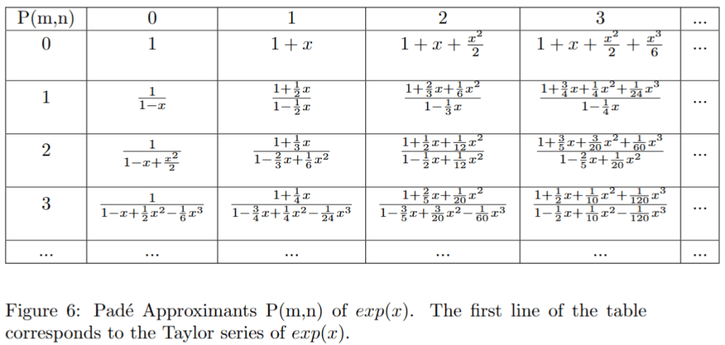
$\displaystyle P(1,1) = \frac{1 + \frac{1}{2} x}{1 - \frac{1}{2} x} = 1 + \frac{x}{1 - \frac{x}{2}}$

Figure 6 shows 16 Padé Approximants for $exp(x)$ . Figure 7 shows $P(0,0)$ , $P(1,1)$ , $P(2,2)$ , $P(3,3)$ and $exp(x)$ .

June 21, 2025
Uniqueness of power series coefficients

The coefficients of the Taylor and Maclaurin series are unique. We are going to demonstrate this assertion because this fact will be very important in the development of the approximation techniques that we want to illustrate in this course.

Consider the power series of the form:

$\displaystyle \sum_{m=0}^\infty a_m (z - z_0)^m$

z and $z_0$ being complex numbers, we will study the convergence of the above power series in the complex plane. If R is the largest radius such that the series converges for all $|z - z_0| < R$ , then R is called the 'radius of convergence'. In its radius of convergence the power series converges to $f(z)$ :

$\displaystyle f(z) = \sum_{m=0}^\infty a_m (z - z_0)^m$

Given function $g(z)$ that is continuous on $C_r(z_0)$ (a circle in the complex plane centred on $z_0$ with radius $r < R$ and oriented counterclockwise):

$\displaystyle g(z)f(z) = g(z) \sum_{m=0}^\infty a_m (z - z_0)^m$

Using the theorem on integration of power series:

$\displaystyle \int_{C_r(z_0)} g(z)f(z) \, dz = \int_{C_r(z_0)} g(z) \sum_{m=0}^\infty a_m (z - z_0)^m \, dz$

$\displaystyle = \sum_{m=0}^\infty a_m \int_{C_r(z_0)} g(z) (z - z_0)^m \, dz$

Defining $g(z)$ :

$\displaystyle g(z) = \frac{1}{2\pi i} \frac{1}{(z - z_0)^{n+1}}$

the integral becomes:

$\displaystyle \int_{C_r(z_0)} g(z)f(z) \, dz = \frac{1}{2\pi i} \int_{C_r(z_0)} \frac{f(z)}{(z - z_0)^{n+1}} \, dz$

Then:

$\displaystyle = \sum_{m=0}^\infty a_m \frac{1}{2\pi i} \int_{C_r(z_0)} \frac{(z - z_0)^m}{(z - z_0)^{n+1}} \, dz$

$\displaystyle = \sum_{m=0}^\infty a_m \frac{1}{2\pi i} \int_{C_r(z_0)} \frac{1}{(z - z_0)^{n-m+1}} \, dz$

Observing that:

$\displaystyle \frac{1}{2\pi i} \int_{C_r(z_0)} \frac{1}{(z - z_0)^{n-m+1}} \, dz = \begin{cases} 1 & \text{for } m = n \\ 0 & \text{for } m \neq n \end{cases}$

the integral becomes:

$\displaystyle \sum_{m=0}^\infty a_m \frac{1}{2\pi i} \int_{C_r(z_0)} \frac{(z - z_0)^m}{(z - z_0)^{n+1}} \, dz = a_n$

Using the Cauchy formula for a holomorphic function:

$\displaystyle \frac{f^{(n)}(z_0)}{n!} = \frac{1}{2\pi i} \int_{C_r(z_0)} \frac{f(z)}{(z - z_0)^{n+1}} \, dz$

We have:

$\displaystyle \int_{C_r(z_0)} g(z)f(z) \, dz = \frac{1}{2\pi i} \int_{C_r(z_0)} \frac{f(z)}{(z - z_0)^{n+1}} \, dz$

$\displaystyle \int_{C_r(z_0)} g(z)f(z) \, dz = a_n$

From Cauchy formula:

$\displaystyle \boxed{a_n = \frac{f^{(n)}(z_0)}{n!}}$

Therefore, the given power series is exactly equal to the Taylor series for $f(z)$ about the point $z_0$ and the coefficients are unique. The uniqueness of coefficients of Taylor and Maclaurin series will be used for solving very hard or even impossible-to-solve-exactly-problems with perturbation theory.

June 20, 2025
Some observations on functions
After looking at numbers, we will continue with a few practical observations about functions. The Taylor series of a real or complex-valued function $f(x)$ that is infinitely differentiable at a real or complex number $a$ is the power series:

$\displaystyle f(x) = f(a) + \frac{f'(a)}{1!} (x-a) + \frac{f''(a)}{2!} (x-a)^2 + \frac{f'''(a)}{3!} (x-a)^3 + \cdots$

$\displaystyle = \sum_{n=0}^{\infty} \frac{f^{(n)}(a)}{n!} (x-a)^{n}$

Using $a = 0$ , we obtain the so-called Maclaurin series:

$\displaystyle f(x) = f(0) + \frac{f'(0)}{1!} x + \frac{f''(0)}{2!} x^2 + \frac{f'''(0)}{3!} x^3 + \cdots$

$\displaystyle = \sum_{n=0}^{\infty} \frac{f^{(n)}(0)}{n!} x^{n}$

The series above are clearly “power series” since we could write them as:

$\displaystyle a_0 + a_1 (x-a) + a_2 (x-a)^2 + a_3 (x-a)^3 + \cdots$

and

$\displaystyle a_0 + a_1 x + a_2 x^2 + a_3 x^3 + \cdots$

respectively, using the definition $a_n = \frac{f^{(n)}(a)}{n!}$ for the Taylor series or $a_n = \frac{f^{(n)}(0)}{n!}$ for the Maclaurin series.

The Taylor series of a polynomial is the polynomial itself.

Taylor and Maclaurin series can be used in a practical way to program functions in a calculating machine or computer. A function such as $\texttt{cos(x)}$ or $\texttt{sin(x)}$ etc. has no meaning for a computer. For a computer, $\texttt{cos(x)}$ and $\texttt{sin(x)}$ are just symbols with no explicit algorithm defined to compute numerical results. Here are some Maclaurin series of important functions:

$\displaystyle \frac{1}{1-x} = \sum_{n=0}^{\infty} x^n, \quad x \in (-1,1)$

$\displaystyle \frac{1}{(1-x)^2} = \sum_{n=1}^{\infty} n x^{n-1}, \quad x \in (-1,1)$

$\displaystyle \frac{1}{(1-x)^3} = \sum_{n=2}^{\infty} \frac{(n-1)n}{2} x^{n-2}, \quad x \in (-1,1)$

$\displaystyle e^{x} = \sum_{n=0}^{\infty} \frac{x^n}{n!}$

$\displaystyle = \frac{x^0}{0!} + \frac{x^1}{1!} + \frac{x^2}{2!} + \frac{x^3}{3!} + \frac{x^4}{4!} + \frac{x^5}{5!} + \cdots$

$\displaystyle = 1 + x + \frac{x^2}{2} + \frac{x^3}{6} + \frac{x^4}{24} + \frac{x^5}{120} + \cdots, \quad x \in \mathbb{R}$

$\displaystyle \ln(1+x) = \sum_{n=1}^{\infty} \frac{(-1)^{n+1}}{n} x^{n}$

$\displaystyle = x - \frac{x^2}{2} + \frac{x^3}{3} - \frac{x^4}{4} + \cdots, \quad x \in (-1,1]$

$\displaystyle \sin x = \sum_{n=0}^{\infty} \frac{(-1)^n}{(2n+1)!} x^{2n+1}$

$\displaystyle = x - \frac{x^3}{3!} + \frac{x^5}{5!} - \frac{x^7}{7!} + \frac{x^9}{9!} - \frac{x^{11}}{11!} + \cdots, \quad x \in \mathbb{R}$

$\displaystyle \cos x = \sum_{n=0}^{\infty} \frac{(-1)^n}{(2n)!} x^{2n}$

$\displaystyle = 1 - \frac{x^2}{2!} + \frac{x^4}{4!} - \frac{x^6}{6!} + \frac{x^8}{8!} - \frac{x^{10}}{10!} + \cdots, \quad x \in \mathbb{R}$

For programming the sine function we could use, for example, the series above as follows (in Python):
```
def sin(x):
    epsilon = 1e-16
    term = x
    sine = x
    sign = -1
    n = 1
    while abs(term) > epsilon:
        term *= x * x / ((2 * n) * (2 * n + 1))
        sine += sign * term
        sign *= -1
        n += 1
    return sine
```
June 15, 2025
Some observations on numbers
The aim of this section is to get us used to using geometric series or continued fractions to represent numbers. We will first have a look at some geometric series:

$\displaystyle 2 = 1 + 1$

$\displaystyle = 1 + \frac{1}{2} + \frac{1}{2}$

$\displaystyle = 1 + \frac{1}{2} + \frac{1}{4} + \frac{1}{4}$

$\displaystyle = \cdots$

$\displaystyle = 1 + \frac{1}{2} + \frac{1}{4} + \frac{1}{8} + \frac{1}{16} + \frac{1}{32} + \frac{1}{64} + \cdots$

$\displaystyle = \sum_{n=0}^{\infty} \left(\frac{1}{2}\right)^n$

More generally, we can write a geometric series as:

$\displaystyle S(x) = x^0 + x^1 + x^2 + x^3 + \cdots$

$\displaystyle = 1 + x + x^2 + x^3 + \cdots$

$\displaystyle = 1 + x (1 + x + x^2 + \cdots)$

$\displaystyle = 1 + x S(x)$

Therefore:

$\displaystyle S(x) = \frac{1}{1-x}$

We have to be careful using this formula, since the radius of convergence of $S(x)$ is $(-1, 1)$ and $\frac{1}{1-x}$ is defined on $\mathbb{R} \setminus \{1\}$ . We can consider $\frac{1}{1-x}$ as some “representation” of $S(x)$ on $(-1, 1)$ .

This formula allows us, for example, to find that the argument of the geometric series of 3 is $\frac{2}{3}$ ( $\frac{2}{3} \in (-1, 1)$ ensures convergence of the series):

$\displaystyle 3 = \frac{1}{1-x} \implies x = \frac{2}{3}$

Now we can write $3$ as:

$\displaystyle 3 = \sum_{n=0}^{\infty} \left(\frac{2}{3}\right)^n$

$\displaystyle = 1 + \frac{2}{3} + \frac{4}{9} + \frac{8}{27} + \frac{16}{81} + \frac{32}{243} + \cdots$

Instead of writing numbers as a geometric series, we could also decide to write a number as a continued fraction with the form:

$\displaystyle a_0 + \frac{1}{a_1 + \frac{1}{a_2 + \frac{1}{a_3 + \frac{1}{a_4 + \cdots}}}}$

To calculate the coefficients $a_0, a_1, a_2, \ldots$ , we can use the continued fraction algorithm, which iteratively takes the integer part of the number and inverts its fractional part. In the case of the number $\sqrt{2} \approx 1.41421356$ , we proceed as follows:

$\displaystyle \sqrt{2} \approx 1.41421356, \quad a_0 = \lfloor \sqrt{2} \rfloor = 1$

$\displaystyle \sqrt{2} - 1 \approx 0.41421, \quad \frac{1}{\sqrt{2} - 1} \approx 2.41421, \quad a_1 = \lfloor 2.41421 \rfloor = 2$

$\displaystyle \frac{1}{\sqrt{2} - 1} - 2 = \sqrt{2} - 1 \approx 0.41421, \quad \frac{1}{\sqrt{2} - 1} \approx 2.41421, \quad a_2 = \lfloor 2.41421 \rfloor = 2$

$\displaystyle \frac{1}{\sqrt{2} - 1} - 2 = \sqrt{2} - 1 \approx 0.41421, \quad \frac{1}{\sqrt{2} - 1} \approx 2.41421, \quad a_3 = \lfloor 2.41421 \rfloor = 2$

$\displaystyle \cdots$

The process repeats, leading to the coefficients $a_0 = 1$ , $a_1 = 2$ , $a_2 = 2$ , $a_3 = 2, \ldots$ . Thus, we can write $\sqrt{2}$ as a continued fraction:

$\displaystyle \sqrt{2} = 1 + \frac{1}{2 + \frac{1}{2 + \frac{1}{2 + \cdots}}}$

The convergents of this continued fraction are:

$\displaystyle c_0 = 1$

$\displaystyle c_1 = 1 + \frac{1}{2} = \frac{3}{2} = 1.5$

$\displaystyle c_2 = 1 + \frac{1}{2 + \frac{1}{2}} = 1 + \frac{2}{5} = \frac{7}{5} = 1.4$

$\displaystyle c_3 = 1 + \frac{1}{2 + \frac{1}{2 + \frac{1}{2}}} = 1 + \frac{5}{12} = \frac{17}{12} \approx 1.4167$

$\displaystyle \cdots$

These convergents approach $\sqrt{2} \approx 1.41421356$ . Note that an alternative method, such as associating the partial sums of a geometric series to a continued fraction, often leads to non-standard coefficients (e.g., negative or non-integer values like $-\frac{3}{2}$ for $2$ or $-\frac{4}{3}$ for $\frac{3}{2}$ ), which may cause convergence issues. The continued fraction algorithm ensures integer coefficients and reliable convergence.

To find a continued fraction for $\pi$ , we can use its decimal expansion or a series approximation. For example, we can use the following series:

$\displaystyle \pi = \sum_{n=0}^{\infty} \frac{2^{n+1} n!^2}{(2n+1)!} \approx 3.1415926535\ldots$

Then we proceed as follows:
1. Let $a_0$ be the largest integer that does not exceed $\pi$ , namely $3$ :
  $\displaystyle a_0 = 3$
2. Compute:
  $\displaystyle \pi \approx 3.141592$
  $\pi - 3 \approx 0.141592, \quad \frac{1}{\pi - 3} \approx 7.062513, \quad a_1 = \lfloor 7.062513 \rfloor = 7$
3. Continue iteratively:
  $\displaystyle \frac{1}{\pi - 3} - 7 \approx 0.062513, \quad \frac{1}{0.062513} \approx 15.99659, \quad a_2 = \lfloor 15.99659 \rfloor = 15$
  
  $\displaystyle \frac{1}{0.06251} - 15 \approx 0.99659, \quad \frac{1}{0.996594} \approx 1.003417, \quad a_3 = \lfloor 1.003417\rfloor = 1$
  
  $\displaystyle \cdots$
Using this technique, the continued fraction for $\pi$ is:

$\displaystyle \pi = 3 + \frac{1}{7 + \frac{1}{15 + \frac{1}{1 + \cdots}}}$

The number $\pi$ itself does not appear as a coefficient in this continued fraction. We could also represent $\pi$ (or any real number) using a generalized continued fraction:

$\displaystyle a_0 + \frac{b_1}{a_1 + \frac{b_2}{a_2 + \frac{b_3}{a_3 + \cdots}}}$
June 12, 2025
Motivation

The general idea of this blog is to present mathematical techniques for solving complicated or even impossible-to-solve-exactly problems using approximation methods. In fact, the vast majority of problems encountered in mathematics or physics cannot be solved exactly, and most problems that could be solved exactly have already been solved.

We’ll primarily focus on a technique known as perturbation theory. Informally, perturbation theory is a method for tackling complex problems by reducing them to a sequence of simpler ones.

The basic principle: break a complex problem into many (potentially infinitely many) simpler ones, then “glue” their solutions together to approximate the solution to the original.

Before presenting perturbation theory, we need to develop approximation techniques for summing potentially divergent series. We will therefore begin by presenting various approximation and summation techniques. Our approach is closer to the methods of natural sciences than to the rigorous ‘Theorem-Proof’ style of pure mathematics. This mathematical style, although less rigorous, will enable us to solve problems that are challenging for the rigorous method. In this spirit, our presentation resembles that of a geologist or chemist discovering new minerals or elements: carefully recording observations in a field journal or lab notebook, making sense of what is seen, and developing concepts to address real problems.

In summary, we would like to present analytical approximation methods for solving problems that are difficult or impossible to solve exactly.

This particular approach to mathematics is not new; it has already been described by the great French mathematician Henri Poincaré in Chapter 8 of his book Les méthodes nouvelles de la mécanique céleste (1892). Henri Poincaré begins this chapter with the following comment concerning the summation of series:

“There is a sort of misunderstanding between geometers and astronomers about the meaning of the word convergence. Geometers, preoccupied with perfect rigour and often too indifferent to the length of inextricable calculations, the possibility of which they conceive without thinking of actually undertaking them, say that a series is convergent when the sum of the terms tends towards a given limit, even if the first terms decrease very slowly. Astronomers, on the other hand, are accustomed to saying that a series converges when the first twenty terms, for example, decrease very rapidly, even though the following terms should increase indefinitely.

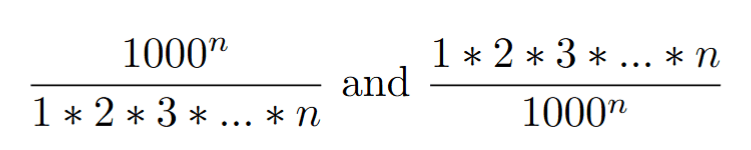
So, to take a simple example, let’s consider the two series with general terms:

Geometers will say that the first converges, and even that it converges rapidly, because the millionth term is much smaller than the 999,999th; but they will regard the second as divergent, because the general term can grow beyond any limit.

Astronomers, on the other hand, will regard the first series as divergent, because the first 1000 terms are increasing; and the second as convergent because the first 1000 terms are decreasing and this decrease is initially very rapid.

Both rules are legitimate: the first, in theoretical research; the second, in numerical applications. Both must prevail, but in two separate domains whose boundaries must be clearly defined.”

Another historical example from theoretical physics vividly illustrates Poincaré’s point. In quantum electrodynamics (QED), the perturbative series expansions are divergent in the “geometer’s” sense. However, by keeping only the first few terms — since calculating further terms becomes prohibitively difficult — physicists obtain predictions that match experimental results with astonishing precision.

In 1965, the Nobel Prize in Physics was awarded to Feynman, Schwinger, and Tomonaga for their groundbreaking work in QED using these techniques. Poincaré would likely have counted them among the “astronomers.”

June 5, 2025